By Mifan Careem
Director - Solutions Architecture, WSO2
The ability to determine or forecast the capacity of a system or set of components, commonly known as 'sizing' a system, is an important activity in enterprise system design and Solution Architecture. Oversizing a system leads to excess costs in terms of hardware resources, while undersizing might lead to reduced performance and the inability of a system to serve its intended purpose. Imagine an e-commerce provider going out of memory on Black Friday or imagine a search engine provider paying 20 times the cost of their optimal server capacity – both scenarios an architect would dread.
The complexity of course is forecasting the capacity to a fair degree of accuracy. Capacity planning in enterprise systems design is an art as much as it is a science. Along with certain parameters, it also involves experience, knowledge of the domain itself, and inside knowledge of the system. In some instances, it goes as far as analyzing the psychology of the system's expected users, their usage patterns, etc.
There are multiple methodologies of carrying out capacity planning. This paper deals with some parameters of capacity planning, with a focus on how factors like concurrency, transactions per second (TPS), work done per transaction, etc. play a role in it. Of course, many other factors could determine the capacity of a system, including the complexity of transactions, latency and external service calls, memory allocation and utilization, etc.
It is a best practice to test the performance of your newer system to see whether it will perform to the expected capacity once you've set up the system as per the capacity planning forecasts.
Let's take a detailed look at some of these parameters. If capacity planning is a common exercise in your line of work, it is good to have a matrix or checkbox of capacity requirements that can be illed in by different types of users.
Generally throughput is deined as the number of messages processed over a given interval of time. Throughput is a measure of the number of actions per unit time, where time can be in seconds, minutes, hours, etc. TPS is the number of atomic actions, in this case ‘transactions’ per second. For a stateless server, this will be the major characteristic that affects server capacity.
Theoretically speaking, if a user performs 60 transactions in a minute, then the TPS should be 60/60 TPS = 1 TPS. Of course, since all concurrent users who are logged into a system might not necessarily be using that system at the given time, this might not be accurate. Additionally, think time of users and pace time comes into consideration as well. But eliminating the above, this can be considered an average of 1 TPS considering users uniformly accessing the system over 60 seconds; this of course means that we can also expect all users coming within a single second which means a 60 TPS max peak load.
Each incoming 'transaction' to a server will have some level of operations it triggers. This would mean a number of CPU instructions would be triggered to process the said message. These instructions might include application processing as well as system operations like database access, external system access, etc. If the transaction is a simple ‘pass through’ that would mean relatively lesser processing requirements than a transaction that triggers a set of further operations. If a certain type of transaction triggers, for example, a series of complex XML-based transformations or processing operations, this would mean some level of processing power or memory requirements. A sequence diagram of the transaction would help determine the actual operations that are related to a transaction.
From a web application perspective, users submit requests, which are then processed at the server side before returned to a user. The user then often waits on the response, and 'processes' it, before submitting again. This delay is the user think time that falls between requests, and can be taken into account when calculating optimum system load. For machine to machine communication, this think time parameter would be relatively lower. For capacity planning, the average think time is useful in arriving at an accurate throughput number.
A system would have a total number of users - this might not affect the server capacity directly, but is an important metric in database sizing for instance. Of these total set of users, a subset of them would be active users - users who use the system at a given time. Usually the active users login to a system, perform some operations and logout; or they just let the system be, which in turn will kick the user out once the session expires (often in 30 minutes or so). Active users might have a session created for each of them, but concepts like garbage collection, etc. would come into effect as well.
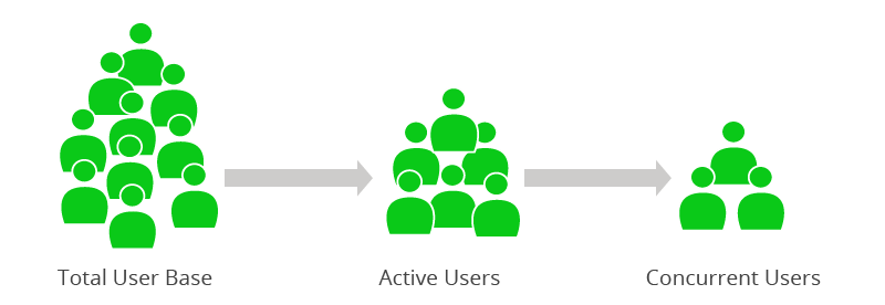
Figure 1: Users in Capacity Planning
Concurrent active users are the number of distinct users concurrently accessing the system at any given time at the same time. As shown in the example in Figure 1, concurrent users are a subset of active users who are using the system at a given time. If 200 active users are logged into the system, and have a 10 second think time, then that amounts to roughly 20 actual concurrent users hitting the system. In capacity planning, this has several meanings and implications. In an application server with a stateful application that handles sessions, the number of concurrent users will play a bigger role than in an ESB, which handles stateless access, for instance. For systems designed in such a way, each concurrent user consumes some level of memory that needs to be taken into account.
Conventionally, a system’s throughput increases with the number of concurrent users until it reaches peak capacity as shown in Figure 2; from then onwards the system would experience performance degradation. Thus, it is important to calculate the maximum concurrency a system can handle.
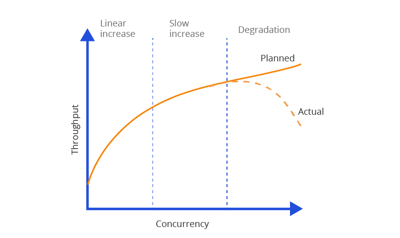
Figure 2: Server Performance - Throughput
The size of the message passed across the 'wire' is also an important factor in determining the required capacity of a system. Larger messages mean more processing power requirement, more memory requirements, or both. As a basis for capacity planning, the following message sizes can be considered.
| Message size range | Message size category |
| Less than 50 KB | Small |
| Between 50 KB and 1 MB | Moderate |
| Between 1 MB and 5 MB | Large |
| Larger than 5 MB | Extra Large |
Figure 3: Message Sizes
Latency is the additional time spent due to the introduction of a system. Non-functional requirements (NFRs) of a system would usually indicate a desired response time of a transaction that a system must then strive to meet. Considering the example in Figure 1, if a single transaction performs a number of database calls, or a set of synchronous web service calls, the calling transaction must 'wait' for a response. This would then add to the overall response time of that said transaction or service call.
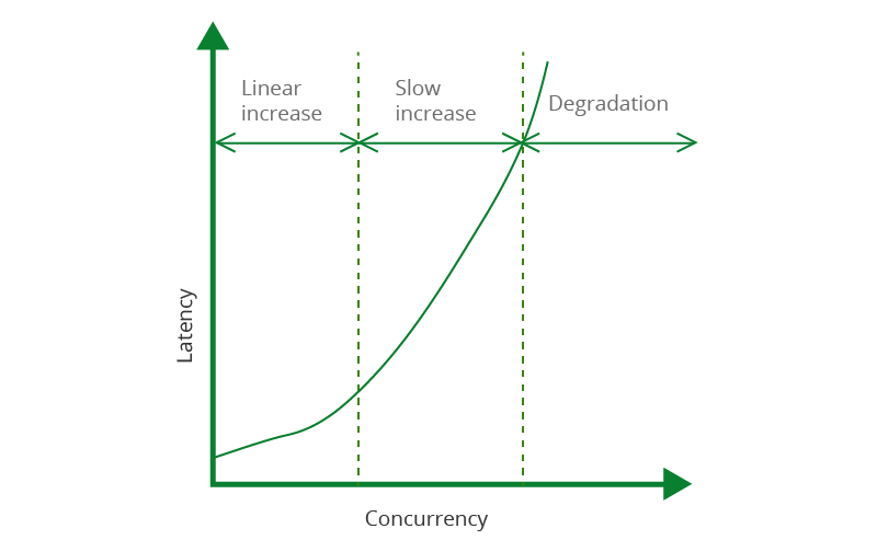
Figure 4: Server Performance - Latency
Latency is usually calculated via a step-by-step process – irst test response times without the newer systems in place, and then test response times with the addition of the newer systems. The latency vs functionality due to the newer systems is then a tradeoff decision. Techniques like caching can be used to improve latency times.
Latency is usually from the client and needs to account for network/bandwith overheads as well.
The QoS requirements, along with other non-functional requirements, would have an effect on how you do capacity planning. For instance, if guaranteed delivery in messaging is required or the transmission of secure messages is a requirement, this would affect the overall performance of the system and needs to be taken into account. Similarly, if the solution is made up of multiple systems with multiple throughput capacities, then some level of throttling needs to be done between those systems.
Another aspect to be considered is the system’s availability or uptime. In theory, the availability is deined as the percentage of system availability in a year. Note though that availability and uptime are not synonymous - the system can be up and running, but might not be available to accept requests, in which case the system is unavailable.
Accepted system downtime is a practical requirement, often found as part of the nonfunctional requirements. This directly determines how a system’s high availability needs to be designed. When calculating capacity, it is important to factor for planned downtime, such as system upgrade and application deployment, and unplanned downtime, such as server crashes.
The availability of a system is determined by the following equation, which yields a percentage result.
x = (n - y) * 100/n
where 'n' is the total number of minutes in a given calendar month and 'y' is the total number of minutes that service is unavailable in a given calendar month.
| Availability(%) | Downtime per year | Downtime per month | Downtime per week |
| 90% ("one nine") | 36.5 days | 72 hours | 16.8 hours |
| 95% | 18.25 days | 36 hours | 8.4 hours |
| 97% | 10.96 days | 21.6 hours | 5.04 hours |
| 98% | 7.30 days | 14.4 hours | 3.36 hours |
| 99% ("two nines") | 3.65 days | 7.20 hours | 1.68 hours |
| 99.5% | 1.83 days | 3.60 hours | 50.4 minutes |
| 99.8% | 17.52 hours | 86.23 minutes | 20.16 minutes |
| 99.9% | 8.76 hours | 43.8 minutes | 10.1 minutes |
| 99.95% | 4.38 hours | 21.56 minutes | 5.04 minutes |
| 99.99% ("four nines") | 52.56 minutes | 4.32 minutes | 1.01 minutes |
Figure 5: Availability Numbers
Source: Wikipedia - https://en.wikipedia.org/wiki/High_availability
With the above concepts (Figure 5) in place, the business needs to decide what the forecasting period should be as well. Are you just focusing on year 1? Will the capacity requirements double in year 2, and if so would there be a signiicant downtime at the end of year one to accommodate this? A table, such as the one given in Figure 6, would be useful for forecasting, and can be based on past trends and future business forecasting.
| Parameter | Year 1 | Year 2 | Year 3 | Year 4 |
| TPS | 50 | 500 | 1000 | 2500 |
| Concurrent Users | 20 | 100 | 500 | 1000 |
Figure 6: Capacity Forecasting for 4 Years
The design of the application or software plays a big role in capacity planning. If a session is created for each concurrent user, this means some level of memory consumption per session. For each operation, factors such as open database connections, the number of application ‘objects’ stored in memory, and the amount of processing that takes place determine the amount of memory and processing capacity required. Well-designed applications will strive to keep these numbers low or would ‘share’ resources effectively. The number of resources that are conigured for an application also play a role. For instance, for database intensive operations, the database connection pool size would be a limiting factor. Similarly, thread pool values, garbage collection times, etc. also determine the performance of a system. Proiling and load testing an application with tools (e.g. for Java apps, JProiler, JConsole, JMeter, etc.) would help determine the bottlenecks of an application.
Optimization parameters should also be taken into account as part of the solution. Techniques like caching can help improve performance and latency – this needs to be looked at from a broader perspective. If the service responses change often, then caching wouldn't make too much of a difference. The cache warm up time needs to be taken into account as well.
It is advisable to have a buffer capacity when allocating server speciications. For instance, allocate 20-30% more of server speciications to that of the peak NFRs to ensure the system doesn’t run out of capacity at peak loads.
Monitoring tools are ideal to calculate a system capacity. Load tests, application, and server proiling via monitoring and proiling tools can help determine the current capacity fairly accurately and help pre-identify bottlenecks.
The type of hardware makes a difference as well. Traditional physical boxes are fast being replaced by VMs and cloud instances. The ideal way to calculate capacity is to have benchmarks on these different environments. A 4GB memory allocation on a VM might not be the same as a 4GB memory allocation on a physical server or an Amazon EC2 instance. There would be instances that are geared towards certain types of operations as well. For example, EC2 has memory optimized, compute optimized or I/O optimized instances based on the type of key operation.
Scalability is the ability to handle requests in proportion to available hardware resources; a scalable system should ideally handle increase/decrease in requests without affecting the overall throughput.
Scalability comes in two lavors; Vertical scalability or Scale Up, where you increase performance of a server by increasing its memory, processing power, etc. (e.g. performance difference between a 4GB RAM server and an 8GB RAM server) vs Horizontal scalability or Scale Out, where you'd deploy more instances of the same type of server.
Based on the availability requirements we discussed above, we'd need to identify the right high availability model. High availability can be categorized as below:
High availability can be achieved via active-active instances, or active-passive failover instances. In the former's case, the availability is quite high whereas in the active-passive scenario, the failover to the passive node needs manual or automatic intervention. Depending on this, the availability of the latter would reduce.
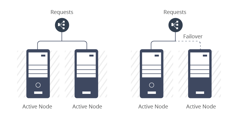
Figure 7: High Availability Within a Data Center
Clustering is a common technique to achieve high availability by providing redundancy at software and hardware level (Figure 7). Typically there are 4 different conigurations that can be used here:
High availability can also be achieved through additional architectural considerations such as
Disaster Recovery (DR) involves the replication of the primary site onto a geographically separate site so that the system can recover when the primary site goes down.
Backup and recovery involves the replication of application, system state and application, and system data onto a backup medium. This can then be recovered either due to primary site failures or due to the application reaching an inconsistent state.
With the cloud, some of the above concepts have been made ubiquitous. The cloud allows servers to be deployed in different geographically separated locations with high speed networks between locations. For instance, Amazon EC2 allows for servers to be deployed within an availability zone, across availability and security zones or across regions, thus providing a very accessible means of achieving full-scale, high availability.
The above are just a few factors that can be used for capacity planning of a system and the importance of these factors vary based on the type of environment.
Different architects use different processes to calculate capacity. A sample process is illustrated in Figure 6; whatever the process, it needs to be coupled with your existing solution architecture process.
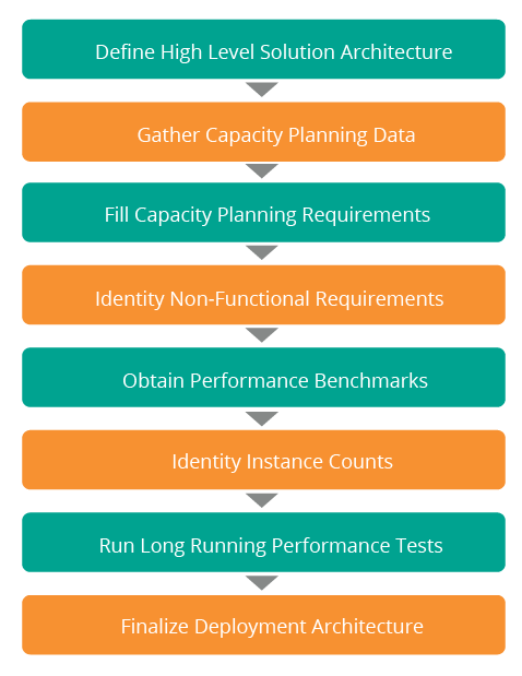
Figure 8: Capacity Planning as Part of Deployment Architecture Process
As per the process shown in Figure 8, it is important to have an accurate business architecture that can be converted into a high-level solution architecture. Based on this, the team can start gathering capacity data that would be used to ill a capacity planning matrix or model.
With these factors in place, we also need a set of benchmark performance numbers to calculate server capacity. For instance, if we know that an enterprise service bus in certain environmental conditions on certain type of capacity performs at 3000 TPS, then we can assume that a server of similar capacity and operations would provide the same.
The table depicted in Figure 9 shows benchmark performance test results of the WSO2 ESB 4.8.1 on speciic environmental conditions.
| WSO2 ESB (4.8.1) Proxy/Transaction Type | TPS* |
| DirectProxy | 4490 |
| CBRProxy | 3703 |
| CBRSOAPHeaderProxy | 4327 |
| CBRTransportHeaderProxy | 5017 |
| XSLTProxy | 3113 |
| SecureProxy | 483 |
Figure 9: WSO2 ESB 4.8.1 Performance Numbers
Source: Wikipedia - https://wso2.com/library/articles/2014/02/esb-performance-round-7.5/
It is key, however, to understand that while benchmarks can be used as a reference model, the applicability of these numbers for your problem domain might vary; therefore, in addition to forecasting capacity, it is important to test the environment to identify its peak capacity.
Without a doubt capacity planning is an art as much as it is a science, and it's clear that experience plays a signiicant role in accurate planning of capacity. In this paper, we've looked at the various concepts of capacity planning and how they affect a solution’s capacity.
Article: ESB Performance Benchmark, Round 7.5
https://wso2.com/library/articles/2014/02/esb-performance-round-7.5/
Whitepaper: WSO2 Carbon Product Performance and Deployment Topology Sizing
https://wso2.com/whitepapers/wso2-carbon-product-performance-and-deploymenttopology-sizing/
Blog: How to measure the peformance of a server:
https://srinathsview.blogspot.com/2012/05/how-to-measure-performance-of-server.html
For more details about our solutions or to discuss a specific requirement