Towards a Precise Definition of Microflows: Distinguishing Short-Lived Orchestration from Workflows

Abstract

A microflow is an artifact for building new application functionality with a graph-based metaphor. This involves creating new functionality by visually representing the flow of control and data between existing functions. Unlike workflows, a flow is deemed "micro" if it is short-lived and imposes fewer quality-of-service demands.

Today, the concept of a microflow lacks a clear definition, leading to confusion when discussing and evaluating associated technologies. This paper proposes a definition to establish clarity regarding the concept of a microflow. We define the essential artifacts required by a language to support microflow specification, highlighting key distinctions between microflows and workflows. We also demonstrate how Business Process Model and Notation (BPMN) facilitates microflow modeling and explore how modern programming languages, such as Ballerina, enable microflow specification. 

1. Microflows and Programming Paradigms 

The predominant use of microflows is to provide new business-relevant functionality by solving integration problems ([1], [2]) in a manner that is considered to be “simpler” than using a traditional programming language. Here, “simpler” means that specifying a microflow should require less programming skills than needed when using a traditional programming language directly. This implies that often a graphical metaphor is supported in specifying a microflow, or at least a syntax is offered that is closer to non-IT savvy users. 

In this chapter, we suggest a definition of the notion of a microflow (section 1.1). Because specifying a microflow, is at the end, some kind of (visual or graphical) programming, we relate constructs well known from programming languages to microflows to better demarcate microflow specifications from traditional programming in section 1.2. 

1.1 A High Level Definition of Microflows 

We suggest the following definition: 

A microflow is an executable specification orchestrating a collection of external functionalities to provide new business-relevant functionality. 

Admittedly, this is an abstract definition. To make this definition more concrete, its ingredients are detailed in what follows: 

• Executable specification: The purpose of a microflow is to realize new business-relevant functionality. It is not about just documenting what should be done. Thus, the description of a microflow has to be precise enough to allow an enactment of the microflow. The enactment may happen by faithfully transforming the microflow into a program that is executed, or by means of an engine that interprets the (visual) description. 
• External functionalities: A microflow makes use of functions that are already available, i.e., that are not provided by the microflow itself, and that are (in this sense) external to the microflow. These functions may have been implemented via various technologies and offered in various formats like microservices, APIs, callable programs, etc. None of these functions realize the new functionality. Thus, these external functions need to be “orchestrated” (see next) to result in the new functionality. The microflow interacts with these functions, e.g., it invokes them or sends messages to them in a structured way.
• Orchestration: The interactions with the external functions used to realize a new business-relevant functionality can not be arbitrary but must take place in an ordered manner. This means that the control flow and the data flow between the external functions, i.e., their orchestration, must be defined. In essence, executing the microflow means to follow these flow definitions making up the orchestration to determine the overall order of interactions with the external functions. The orchestration, thus, integrates the external functions to result in the new functionality. In essence, Specifying a microflow means solving an integration problem. 
• Business-relevant functionality: The orchestration of a microflow defines the order in which the external functionalities are interacted with (control flow) and how the data that these interactions require are exchanged (data flow). This is the integration logic that realizes the new business-relevant functionality. Note that the notion of “business” here is very broad and is by far not restricted to what is typically meant by “business” [4].

The central technical aspect of a microflow is its orchestration, mainly consisting of control flow specifications (see section 2.2) as well as data flow specifications (see section 2.3). Thus, a microflow follows a certain programming paradigm. To position microflows, we briefly remind the major programming paradigms next. 

1.2 Programming Paradigms 

A programming paradigm defines the conceptual building blocks available in a programming language for representing static and dynamic aspects of a program. Static building blocks include variables, records, constants, methods, and classes, for example. Dynamic building blocks encompass assignments, control flow constructs (like sequencing, branching, or iterating), and data flow constructs (like data source, or data sink).

A programming paradigm also recommends how to use the supported building blocks in order to build “a good program”. For example, it may be recommended that each variable should be initialized by a default value, or that each class should have at least one parameterized constructor. A set of building blocks and corresponding recommendations defines a programming style. Fundamentally, there are two classes of programming paradigms, namely imperative and declarative paradigms. This is a coarse classification and a plethora of subclasses of these two paradigms exist.

An imperative paradigm enforces to describe how a problem is to be solved. For this purpose, a corresponding programming language has a state (the set of variables used by the program) and statements (actions that manipulate the state and specifications under which conditions actions take place). An important subcategory of this paradigm is object-oriented programming. It bundles actions and their manipulated states into a single unit (an object). Examples of programming languages supporting an imperative paradigm are C or Java (the latter is also an object-oriented programming language). 

A declarative paradigm requires describing the problem to be solved, not how to solve it. How the problem is solved is derived by the implementation of a corresponding programming language. For example, Prolog allows to describe a problem in terms of expressions of formal logic, and a Prolog interpreter performs logical deduction to compute the solution of the problem. Another example is SQL, which supports describing data manipulations in algebraic expressions, and a SQL interpreter transforms these expressions into imperative code. 

Microflows follow an imperative programming paradigm, focusing on specifying the control flow and the data flow between the external functionalities they integrate. The next section provides details about these constructs for defining these flows. Also, some recommendations are given about the usage of these constructs, i.e., effectively the next section begins to sketch the microflow programming style. Section 3 will explain the most basic relationship between microflows and workflows and will present two languages that can be used to define microflows. Section 4 will expand on the relation between microflows and workflows, discussing additional aspects like interruptibility and transactional capabilities. 

2. Flow Control 

The executable specification of a microflow is in analogy to a musical score, and the external functions are like the musical instruments “orchestrated” by the score. This is the origin of the term orchestration for the executable specification of a microflow, and orchestrator for the execution engine of microflows (or the program generated based on the microflow specification). Most often, the term microflow is used interchangeably for both, the specification of a microflow as well as its execution; only in situations where it is not clear whether the specification or its execution is meant, the terms “microflow specification” and “microflow execution” are used. 

In the following, we will introduce the abstraction of microflows as a graph and its main operational semantics (section 2.1); this graph abstraction reveals the metaphor that can be supported to support business experts in specifying microflows. Next, section 2.2 describes the major control flow features offered by microflows, and section 2.3 sketches a couple of its data flow features. 

2.1 Microflows Are Graphs

When abstracting from concrete syntax (see [5]), a microflow defines a directed graph (see [4] for more details). The nodes of the graph represent the external functions to be interacted with, and the edges define the control flow between these interactions. The nodes, i.e., the representations of the external functions, are referred to as the activities of the microflow (sometimes the terms steps or tasks are used also). An external functionality associated with an activity is called the implementation of the activity. In Figure 1, the activities of the microflow are A, B, and C, and the implementation of activity A, for example, is the external functionality denoted by i(A). 

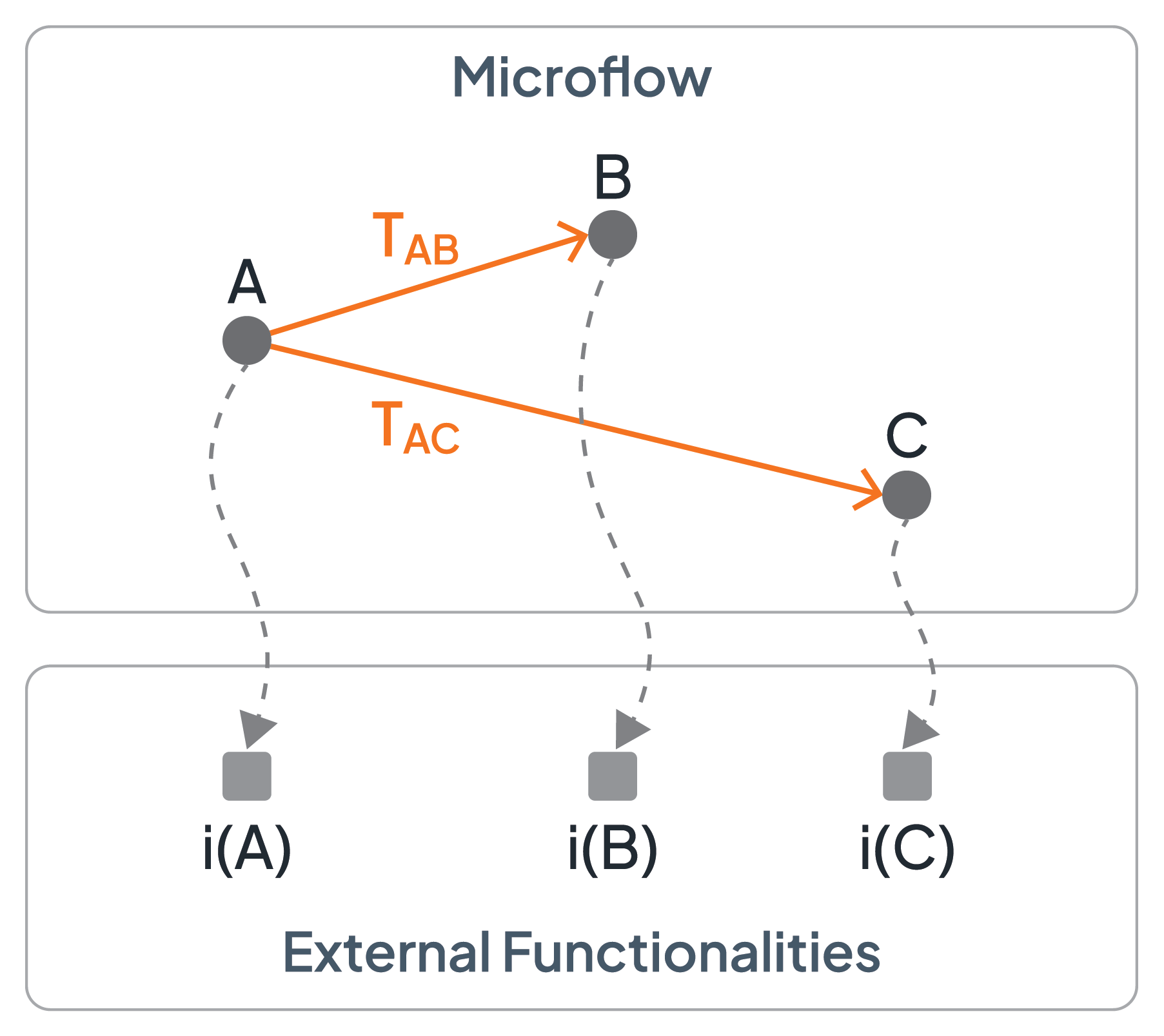
Figure 1: Fundamental Ingredients of the Graph Structure of a Microflow

An edge starting at activity A and ending at activity B has the following operational semantics: as soon as the implementation i(A) of activity A is completed, the edge is followed and the implementation i(B) of the target activity B is activated (for brevity, it can be stated that activity A completes or B is activated having in mind that the implementations of the activities are completed or are activated). The edges control the flow between the activities and are, thus, called control flow connectors. In addition, a control flow connector has a condition associated with it, its so-called transition condition: if and only if this transition condition is evaluated to true (once the startpoint activity of the control flow connector is completed) its control flow connector will be followed and the endpoint activity of the control flow connector will be activated. In case the transition condition evaluates to false, the control flow connected will not be followed and, thus, the endpoint activity will not be reached and will consequently not be activated (and the control flow is stalled along this path of the graph). If no explicit transition condition is defined for a control flow connector, a constant “true” condition is assumed. Thus, the transition conditions determine which paths are actually taken through the graph. 

When an activity is reached via a control flow connector, the activity will be activated. This means that the required interaction between the microflow and the activity’s implementation will be performed. For example, interaction with an activity’s implementation can mean to synchronously invoke the implementation; to asynchronously send a message to it; to wait for a message; and so on. Typically, an activity is annotated with a decorator indicating the type of interaction between the activity and its implementation. For example, Figure 2 depicts three sample decorators (that vary from tool to tool supporting the specification of microflows): activity A interacts synchronously with its implementation, activity B sends out a message, or activity C waits for an incoming message. 

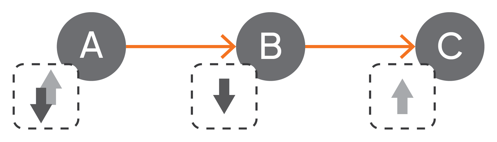
Figure 2: Decorators Indicating Types of Interactions

A transition condition is based on variables of the microflow (see section 2.3 and Figure 11). The variables' values serve as the input and output for both the activities and their implementations (refer to section 2.3, Figures 7 and 10). In other words, these variables are effectively manipulated when activity implementations return data. As a consequence, the truth value of the transition conditions is affected by the activity implementations’ outputs, and, thus, different runs of a microflow result in different values of these variables, which, in turn, result in different paths taken through the graph of the microflow. 

An activity may have multiple outgoing control flow connectors defined. As a consequence, the execution of a microflow may not just be a strict sequence of activities but a partial order: all endpoints of outgoing control flow connectors might be interacted with in parallel. However, only those connectors whose transition conditions evaluate to true will be followed. Thus, any subset of outgoing control flow connectors may be followed, implying that any subset of immediate successors of a completed activity can be interacted with in parallel. 

2.2 Control Flow Artifacts 

The graph metaphor of a microflow supports specifying a variety of basic control flow structures (see Figure 3) that are typically combined to realize more comprehensive control flows. Part 1 of the figure shows how to realize a sequence of activities: activity B succeeds activity A; more precisely, as soon as the implementation i(A) of activity A completes, the implementation i(B) of activity B will be activated. A conditional execution of an activity is depicted in part 2: after completion of activity A, activity B will be activated if and only if the transition condition TAB is true. The graph fragment of an alternative execution is given in part 3: if the transition condition T is true, activity B will be activated, and if the transition condition is false (i.e., ￢T is true), activity C will be activated; this structure is also referred to as an exclusive split of the control flow. Finally, part 4 presents (potential) parallelism: in case both, T_AB as well as T_AC are evaluated to true, both activities A and B will be activated in parallel; if only one of the transition conditions become true, only the corresponding activity is activated, and if none becomes true, none of the activities will be activated - this split is called an inclusive split. 

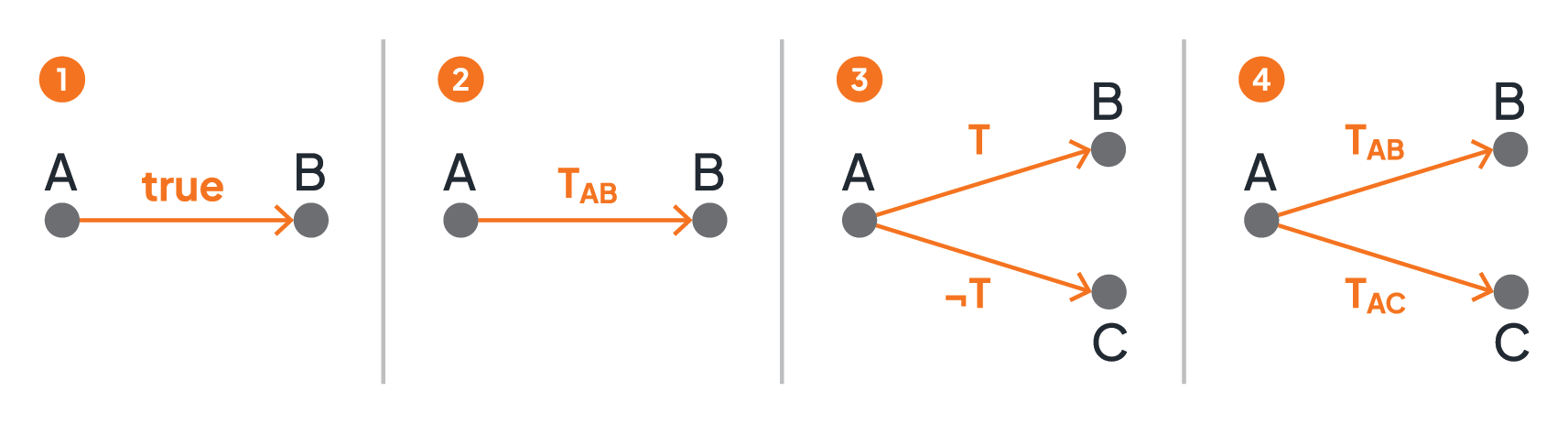
Figure 3: Basic Control Flow Structures - Sequence and Split

Figure 4 presents loop structures as graph fragments. Part 5 shows an until loop: activities A and B as well as all activities between A and B (the loop body) will be iteratively executed as long as the transition condition T is false. A while loop is depicted in part 6: the loop body (i.e., activities A, B, and all activities in between) will be iteratively executed in case the transition condition T is true. 

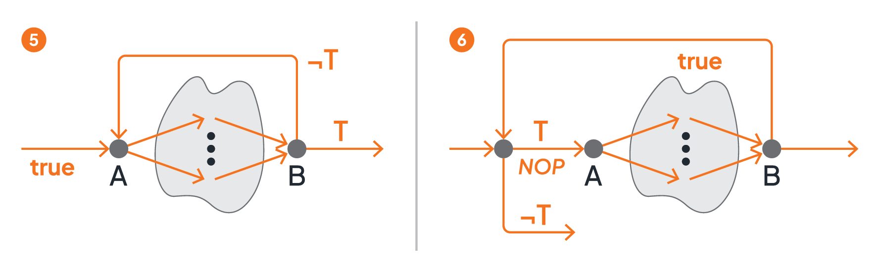
Figure 4: Loop Structures

A graph with such loop structures (i.e., control connectors pointing “backwards”) can become confusing and difficult to understand. To allow simpler graph structures, subflows (for brevity, instead of submicroflows) may be supported: in Figure 5 activity S in part 7 hides a fragment of the graph that is effectively the loop body. In other words, S is a placeholder for the collapsed subflow. The subflow is still a part of the surrounding microflow. As such, the subflow has access to all variables (see section 2.3) of the surrounding microflow, i.e., collapsing is only a visual simplification. The subflow will be iterated until the condition T becomes true. 

In contrast, part 8 of Figure 5 shows the same microflow but as an external functionality, i.e., not as a collapsed fragment of the graph. The microflow M is a standalone implementation that implements activity S, i.e., M = i(S). As a standalone implementation, M has no access to the variables of the parent microflow. When activity S is activated, all required data must be exchanged with the microflow M, as with any other implementation of an activity. Being not part of another microflow, the microflow M can be the implementation of activities of any other microflow, i.e., a microflow is also a reusable artifact. 

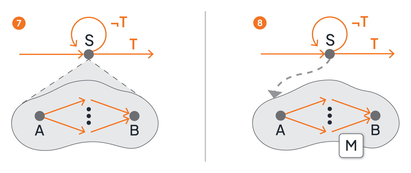
Figure 5: Subflows and Loops

While Figure 3 shows, in part 3 and part 4, the two main control flow structures for splitting a control flow (i.e., an exclusive split in part 3, and an inclusive split in part 4), Figure 6 depicts the major control flow structures for joining independent branches of the control flow. Part 9 is an exclusive join: depending on the truth value of the transition condition T, only one branch of the control flow is taken once the split activity F (also called a fork) completes. Thus, the join activity J is activated as soon as one of its incoming control flow connectors is evaluated to true. Part 10 is an inclusive join: depending on the truth values of the transition conditions T1 and T2, both branches leaving the split activity F will be taken, or only one of the branches, or none. Consequently, considering the activation of the join activity J needs to take care which of its incoming control flow connectors may finally be “reached”: it may occur that a path originating at F encompasses a transition condition that is evaluated to false, i.e., the corresponding path is “dead” and the corresponding incoming control flow connector will never be reached and, thus, is not to be considered when deciding to activate J or not.

If and only if the transition conditions of all control flow connectors that reached J are evaluated to true, activity J is activated. 

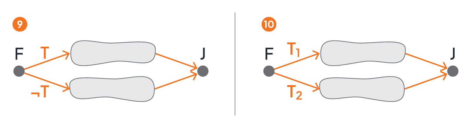
Figure 6: Joining Branches of Control Flow

2.3 Data Flow Artifacts 

Each microflow has a set of variables assigned, sometimes called the variable pool of the microflow. In Figure 7, these variables are denoted by v₁,...,v_n at the top of the figure. This variable pool is a data flow artifact. Each activity has an input data object and an output data object associated with it, like I(A) and O(A) denote the input data and output data objects of activity A in the figure. These data objects are data flow artifacts too, and the association of data objects to activities (dashed arrows between data objects and activities) is yet another data flow artifact. 

Input data objects are materialized from the variable pool at the time the activity is to be activated. This means that the current values of the variables of the pool are used as values of the parameters of the input data object of the activity. Materializing an input data object may be as simple as copying data values from the pool to parameters of the input data object, or it may involve a more complex assignment, which is another data flow artifact (the star shapes with an “×” in Figure 7). Such an assignment may transform values of variables from the pool to become a value of an input parameter of the input data object of the activity. Especially, assignments may compose (e.g., concatenate, compute) values of variables to result in values of parameters. In case no transformation is required, the parameters of the input data object of an activity may simply refer to the corresponding variables from the pool by name. For example, the input data I(A) in Figure 7 consists of parameters p₁, p₂, and p₃, which are materialized from the variable pool by the assignment X1.

An assignment may also transform values of output parameters of the output data object of an activity to values of variables of the pool (i.e., the output data object is dematerialized): assignment X2 in Figure 7 transforms the values of the two parameters q1 and q2 into values of variables from the pool. In case no transformation is required, the output parameters may simply refer to the corresponding variables of the pool by name, resulting in copying the values of the parameters into the variables. 

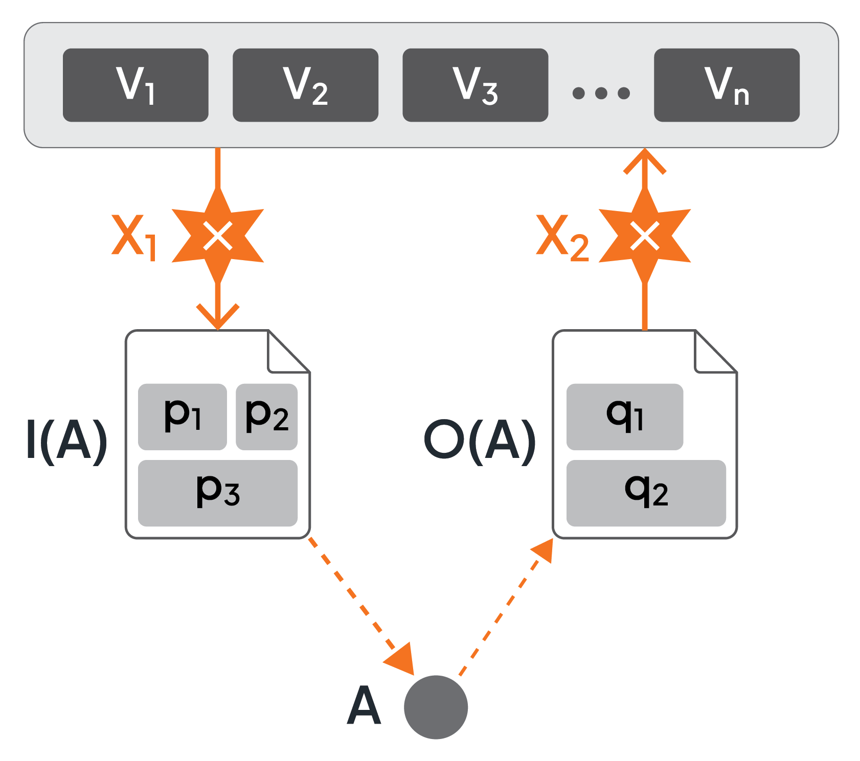
Figure 7: Variable Pool, Data Objects, and Assignments

Some implementations of microflows allow assignments to directly access output data objects of formerly completed activities [4]. As shown in Figure 8, assignment X uses values from both the output data objects O(A₁) and O(A₂) of activities A₁ and A₂, as well the variable pool to materialize the input data object of activity A. This is a powerful feature. It allows dedicated access to values of output parameters of specific activities directly, i.e., without using the values that have been copied to variables of the pool. Whenever an activity completes, the values from its output parameters are copied to the pool, overwriting values that have been copied earlier from output parameters of other activities. In this sense, older values are lost in the variable pool. Retrieving values directly from specific output data objects avoids this loss of older values. But this feature introduces a lot of complications like having to cope with values of output parameters that have not been produced at all because an activity was never activated - see [4]. Because of this, we assume for simplicity that assignments retrieve values of variables from the pool only. 

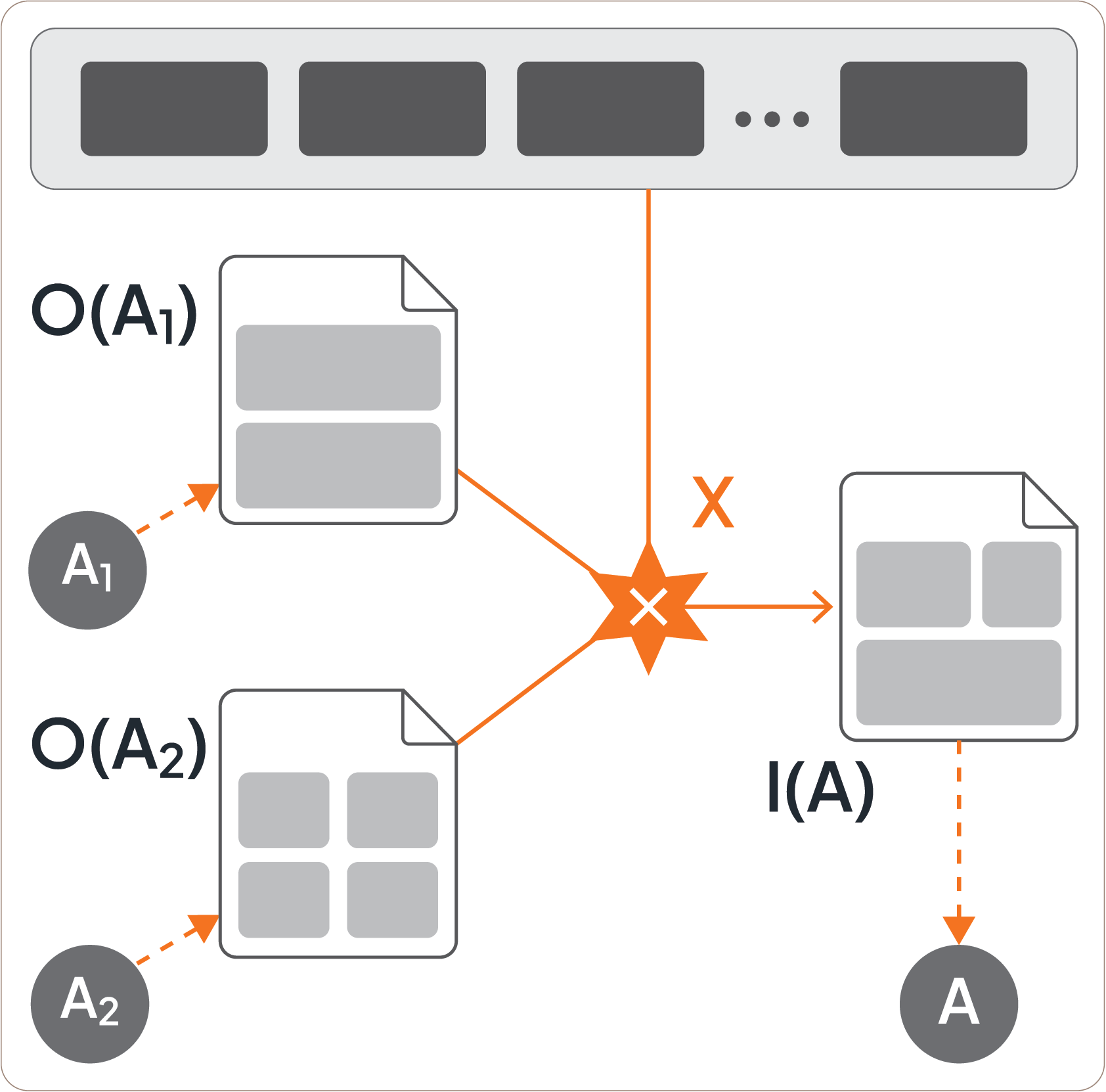
Figure 8: Direct Access to Output Data Objects

Assignments are special data flow artifacts of a microflow. They are defined for each input data object and output data object (if needed). This is convenient and allows to focus on data flow separate from control flow. Some microflow environments (refer to [12]) require to realize assignments as separate activities to be injected before and after the activity consuming the input and producing the output (see Figure 9). This is not the preferred approach since it mixes control flow and data flow unnecessarily, and clutters the microflow with these special kinds of assignment activities that are not natural in terms of the business logic of the functionality to be built. As a side-comment, to indicate that the parameters of the data objects associated with an assignment activity are simply copied from or to the variable pool, respectively, the graphical assignment construct is decorated with an “identity”-symbol (≡) instead of an “×”-symbol (see Figure 9). 

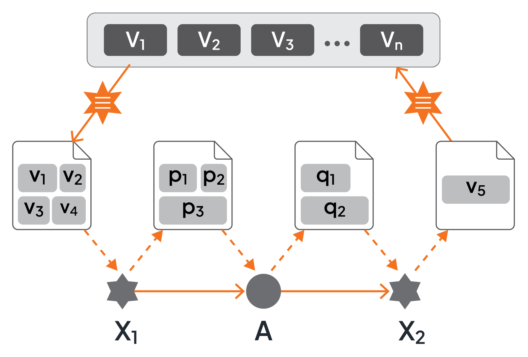
Figure 9: Assignments as Separate Activities

When a microflow interacts with the implementations of its activities, it exchanges data between the microflow and these implementations. Often, a microflow should be independent of the implementations of its encompassed activities, i.e., the implementation should be exchangeable. This is not a problem in case the possible implementations of an activity realize a predefined API [3], since an API specifies the payload of the messages exchanged between the microflow and these implementations. The input data objects and output data objects just correspond to these payloads (see Figure 10 - part 1). 

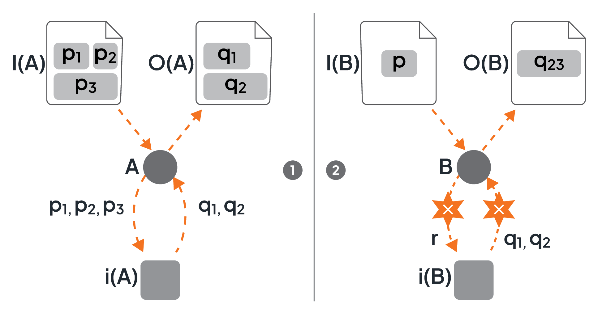
Figure 10: Transforming Input and Output Parameters of an Activity Implementation

In some scenarios, the implementation of an activity may be realized as a program that must be directly interacted with, i.e., this program is not hidden by an API. In this case, several issues must be dealt with, e.g., the type system of the corresponding programming language may be different from the type system of the microflow, or the program may expect further transformations between its signature and the data objects of the activity. Thus, yet another assignment is needed between the activity’s data objects and the input and output parameters of the program (see Figure 10 - part 2). As an example, parameter p of the input data object of activity B may be an integer number, but the implementation i(B) expects this number as a string r; and the output of the implementation i(B) consists of two parameters q₁ and q₂, but the parameter q₂₃ of the output data object expects the two values concatenated. 

Finally, transition conditions have input parameters too. In Figure 11, transition condition T has a set of parameters {pi}. The values of these parameters are materialized based on the values of the variables of the pool. When the values of the parameters of the transition condition require any transformation, a separate assignment must be specified to prepare the data accordingly. The output of a transition condition is always a Boolean value and, thus, requires no transformation at all (not even an explicit specification).

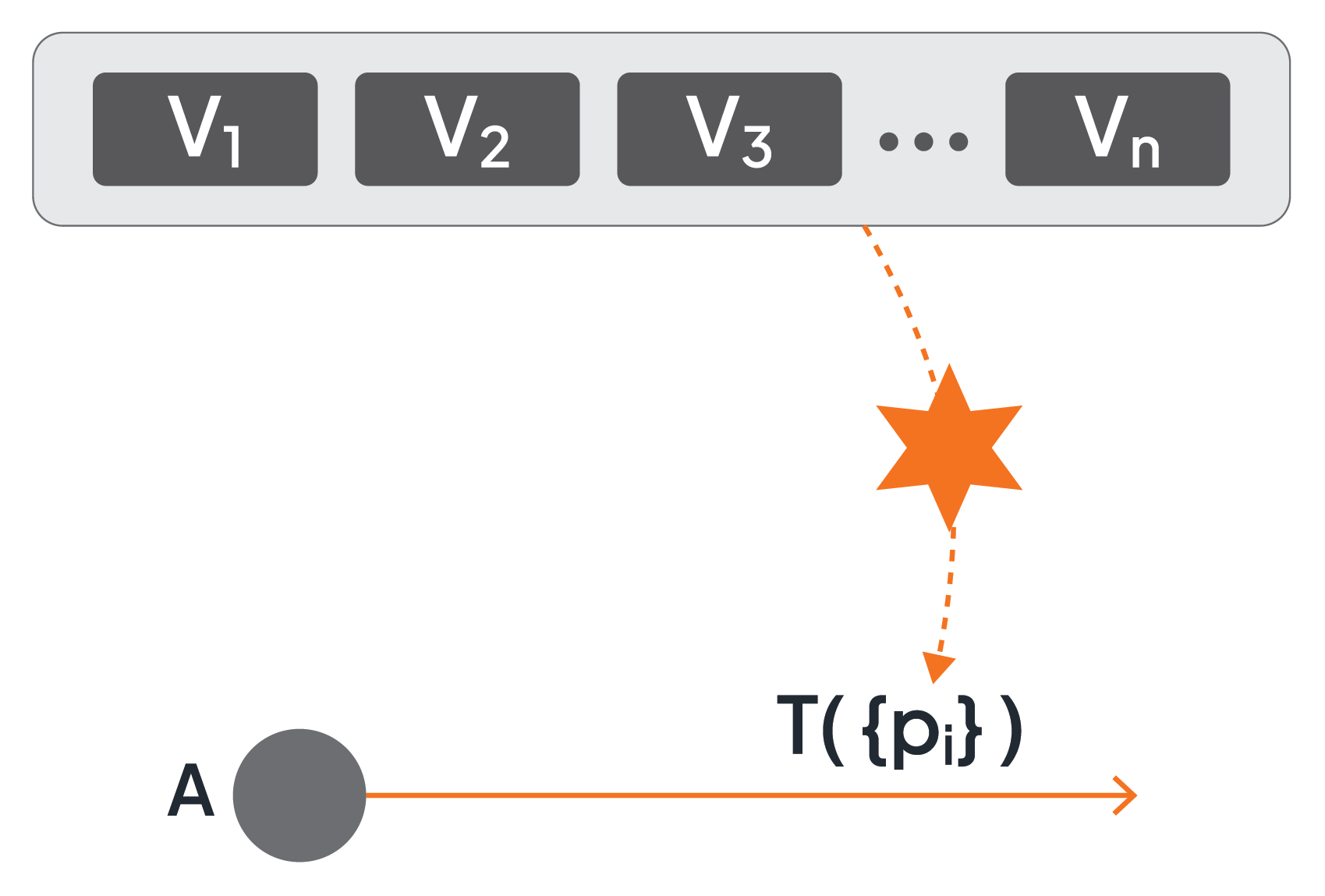
Figure 11: Parameters of Transition Conditions

Another data flow artifact represents external data stores. Figure 12 shows that activity A itself reads input from a data store, and activity B itself writes its output into a data store. The implementations of the activities are assumed to understand how to access the external data stores themselves, i.e., a microflow has no corresponding support as it has for accessing the variable pool by means of assignments. However, if an activity implementation has no capability to access a data store itself, corresponding activities may be injected that read data directly from a store and provide an output data object that contains the data read, and this output data object may be consumed as input of an activity without the capability to directly read data from a data store (and analogously for activities not capable of directly writing to a data store). 

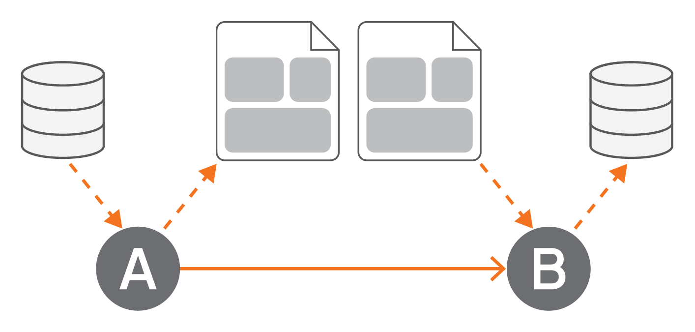
Figure 12: Data Stores as Input or Output of Activities

3. Implementing Microflows

Workflow technology has evolved over decades. Its origin was the IT support of office work, i.e., from forms and document routing to case processing (refer to [4]). The next major step was to enable the management of any kind of business processes. This included the optimization of such processes, which often means to automize (parts of) a process. Fully automated processes basically integrate programs, which, in turn, resulted in the use of workflow technology for orchestrating services (see [9], [12]). It is this integration capability of workflow technology that is at the heart of microflows, i.e., workflow systems may be exploited to realize microflows. 

3.1 Three Dimensions of Workflows

A workflow represents a business process and most often, both terms are used interchangeably. Although, sometimes a small nuance in emphasis is made. The term “workflow” is used to emphasize the realization of a business process in an IT environment, while the term “business process” is used to emphasize its proper business aspects independent of any IT implementation. 

At a very high level, the lifecycle of a workflow is split into two phases: its build time and its runtime. During build time a workflow is basically modeled with a graphical tool, and during runtime, such a model is executed (note that both phases are further refined - see [4] for details about the subjects in this section). A corresponding graphical modeling tool has the goal to support non-IT experts to specify all business aspects of a workflow. This implies that (at least) the three elemental aspects of a business process are supported: what has to be done, who has to do it, and which tools can be used. Metaphorically, the three aspects of “what”, “who”, and “which” are referred to as the three dimensions of a workflow (model), also called the W3-cube. 

The “what” dimension corresponds to the activities to be performed in a business process, and the control flow and the data flow between these activities. The constructs discussed in chapter 2 are supported by a corresponding modeling tool. The organizational structure supporting the business process, i.e., the departments, the employees, and their roles are reflected in the “who” dimension: it specifies who is in charge or who has the capabilities to perform a certain activity. Finally, the execution of an activity is most often supported by a tool, and in the context of digitalization these tools are programs: the association of an activity with a program is fundamentally the “which” dimension. In a nutshell, a business process specifies what activity has to be done by whom and with which tool in a certain context. Note, that the context is basically determined by the transition conditions that are evaluated in the actual data of the business process. More details of workflow technology as it relates to microflows are given in chapter 4. 

A final note on the plethora of terms in this domain: the term “orchestration” is used in case all activities of a workflow are executed automatically, i.e., without involving a human at all. In this case, a workflow is an artifact that integrates a collection of programs. Originally, the term “orchestration” was coined for integrating or aggregating (web) services [12]. In B2B scenarios, business processes of various partners must be stitched together into an artifact of intertwined business process; the term “choreography” has been established for such an artifact. This in turn implied the need for a name for business processes that are standalone, i.e., not intertwined with other business processes (basically a business process involving only organizational elements of a single company): unfortunately, the term “orchestration” has been established for these kinds of business processes, resulting in potential confusion. Also, when workflow technology is exploited in specialized domains, new terms - like process-aware information systems - are coined contributing to terminological confusion (but remember: “A rose is a rose is a rose”). 

3.2 Building Microflows with BPMN

BPMN is a graphical language to model business processes [15]. Its operational semantics, i.e., how its graphical elements are to be interpreted in order to result into a particular running business process, has been influenced by Business Process Execution Language (BPEL) [12]. Once a business process has been modeled by a corresponding modeling tool (e.g., [17]) it must be imported into a BPMN workflow engine (e.g., [18]); after that, the model can be instantiated and executed by the workflow engine several times (with different variable values).

In this section, we sketch how BPMN supports the key control flow features of microflows (see section 2.2). BPMN also offers data flow capabilities (see section 2.3) that we only mentioned briefly: BPMN has constructs for data objects that make up the variable pool of the workflow. Data objects can be associated with activities as their input and output. Input and output data of activity implementations can be defined separately as data input and data output. Assignments are separate artifacts but without a graphical representation. Messages represent data exchanged between the workflow and the outside world.

Briefly, Figure 13 summarizes some of the data flow features. Activity A has input data object I(A) and output data object O(A), and it writes data into a data store (compare also Figure 12). The input data object has parameters p1, p2, p3, and the output data object has parameters q1, q2. These parameters are not represented as graphical artifacts but are specified separately in corresponding forms (see the right side of the figure). The icon of activity A has a decorator in the upper left corner: these are two overlapping gears that specify that activity A is a “service”; the endpoint where the service is offered is given in the “type” field on the form at the right side. 

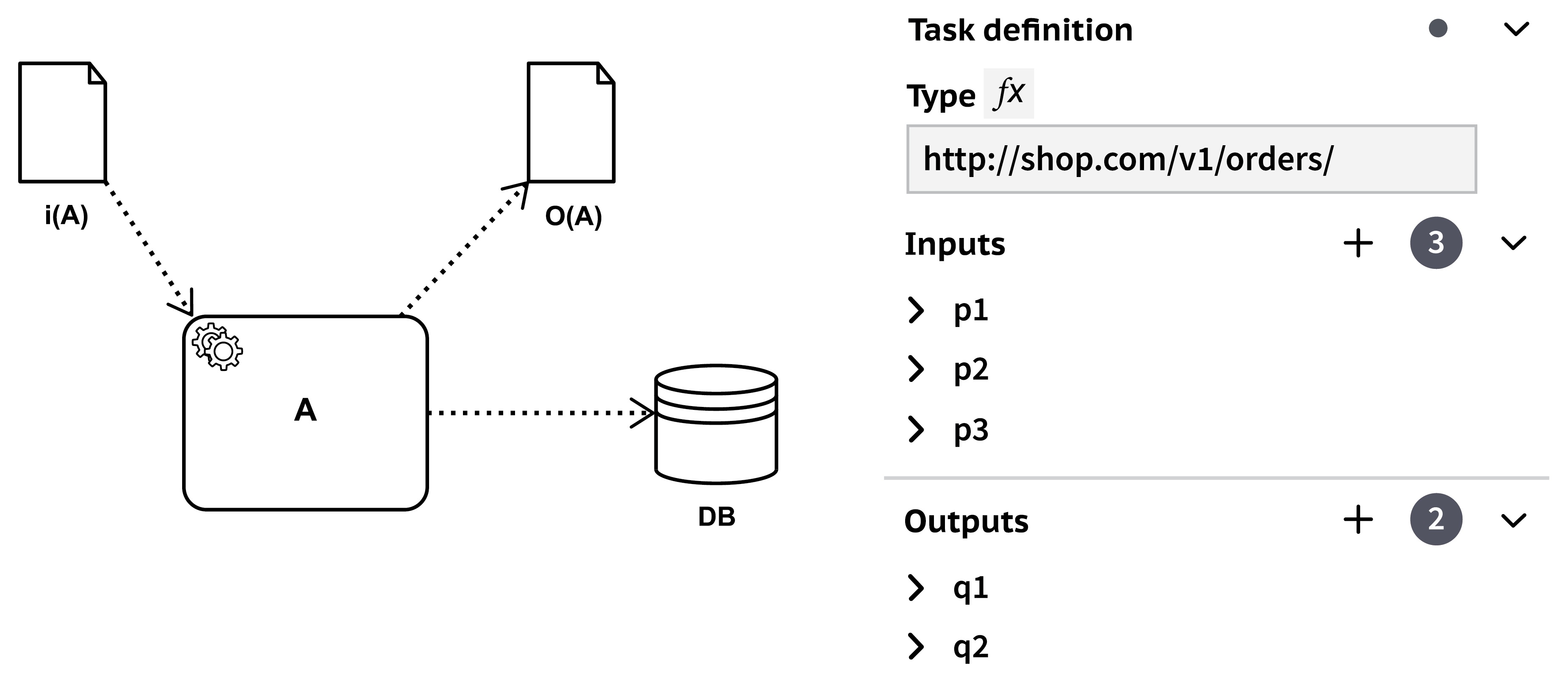
Figure 13: Some Data Flow Features

A few other decorators are shown in Figure 14 (compare also Figure 2). The solid envelope indicates an activity that is just sending a message, and the hollow envelope indicates that the activity is waiting for a message and just consumes it once it arrives. 

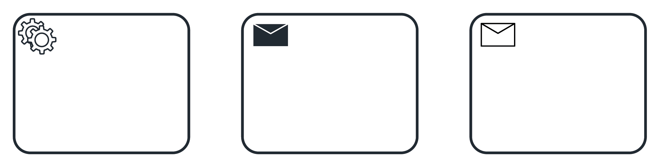
Figure 14: Some Activity Decorators

In Figure 15 (compare the generic representation in Figure 3 part 1) activities A and B are performed in a sequence. Note the circles that are embracing the sequence: the circle with a thin line indicates the start of the microflow, the circle with the thick line indicates the end of the microflow. This is similar to microflows in Ballerina that are discussed in section 3.3 (and see Figure 24). 

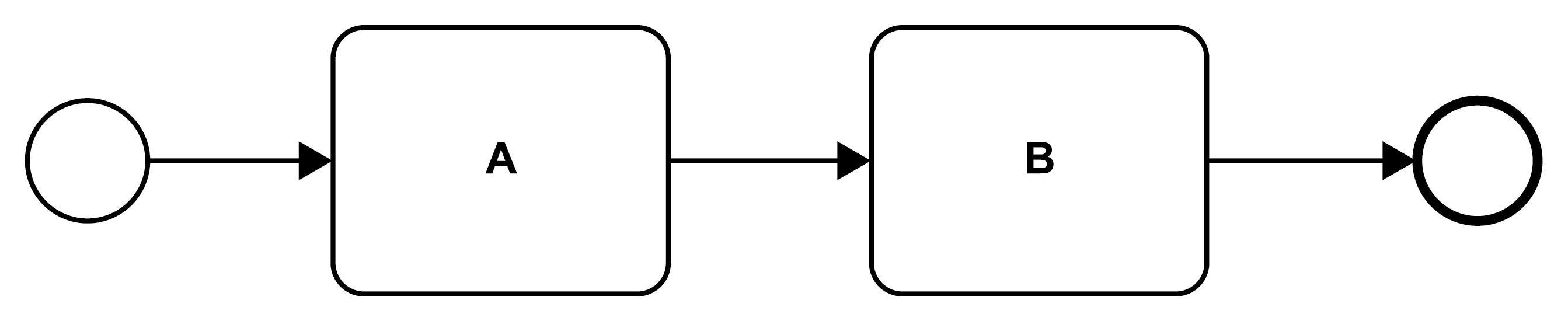
Figure 15: A Sequence of Activities

In contrast to a sequential execution, activities may be run in parallel (see Figure 16). The figure depicts an unconditional parallel split of the control flow, also known as an AND split, i.e., activities A and B will run concurrently. The diamond in the figure is called in BPMN a gateway, and the “+” in the diamond indicates that the control flow is split into parallel paths. There are gateways that branch the control flow into alternate paths by selecting exactly one of the control flow connectors leaving the gateway (decorating the diamond with a “⤫” - see Figure 18), or by selecting any subset of the control flow connectors leaving the gateway (decorating the diamond with an “○” - see Figure 19).

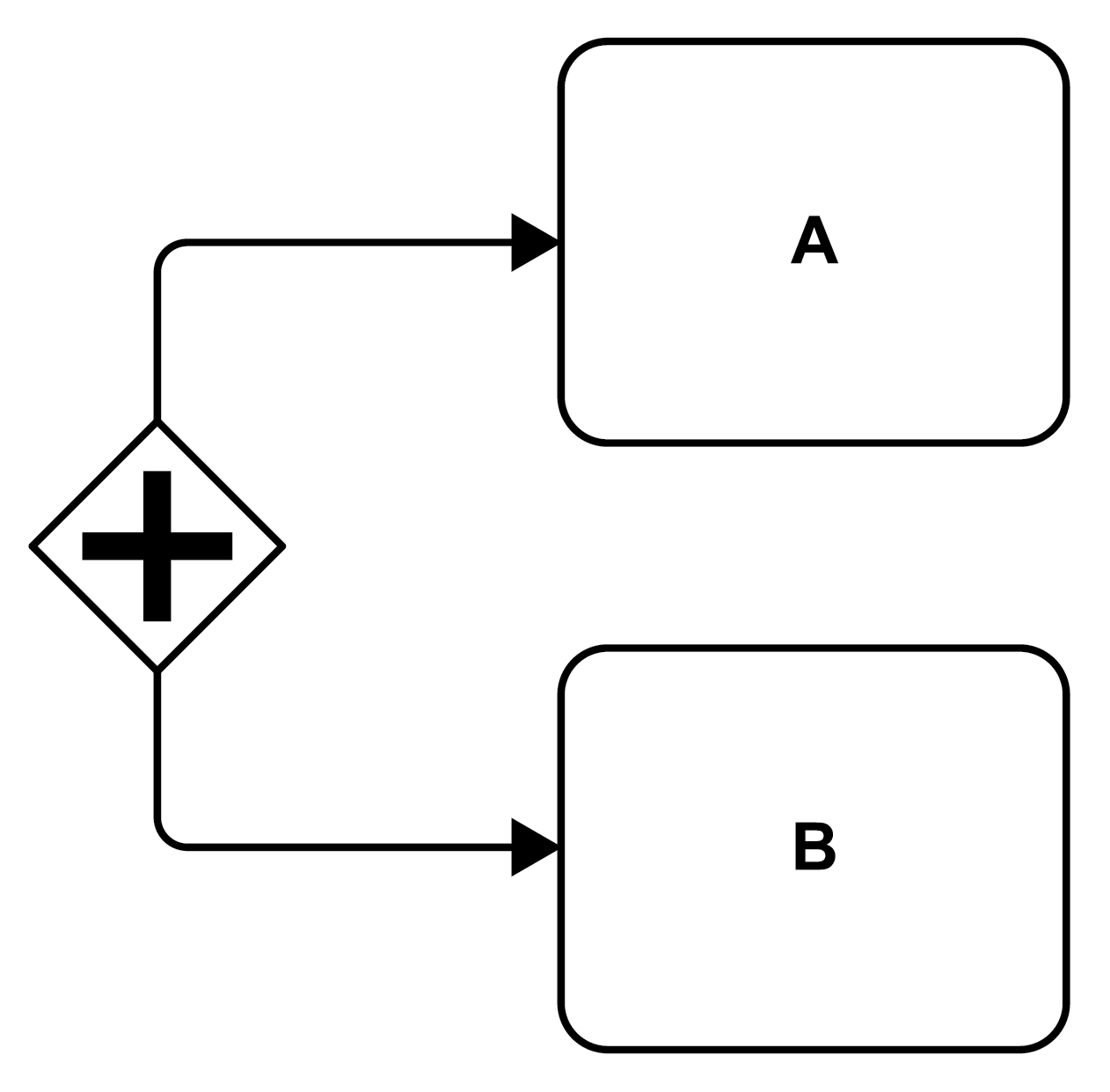
Figure 16: Parallel Activities via a Parallel Split (AND Split)

Control flow connectors may be associated with transition conditions like in Figure 17 (compare the generic representation in Figure 3 part 2). The condition is then shown with the connector, and in addition, the connector may be decorated by a small diamond to indicate that the connector is followed if and only if the condition is true. In the figure, once activity A is completed the transition condition is evaluated (i.e., it is checked whether the value of the Price parameter is less than 100). If the condition is met, activity B will be executed; if the condition is not met, activity B will not be executed and the control flow stops along this actual path.

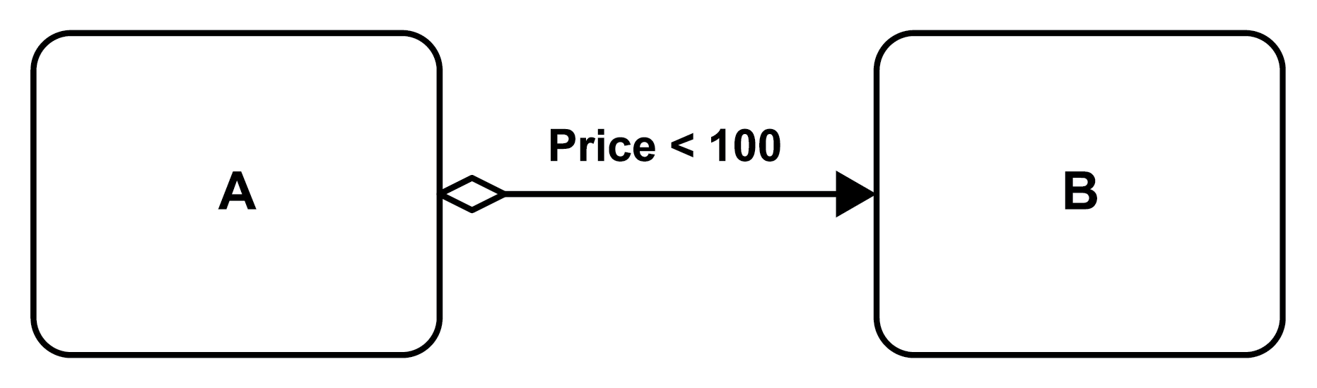
Figure 17: A Conditional Execution of an Activity

Alternative branches of a control flow, i.e., its exclusive split, can be specified by a gateway that is associated with a condition and that is depicted by a diamond decorated by a “⤫” as shown in Figure 18 (compare the generic representation in Figure 3 part 3). In the figure, after activity A completes, the condition associated with the gateway (Price < 100) is evaluated; if it is evaluated to “true” the corresponding path is taken and activity B is performed, otherwise the path decorated with “false” is taken and activity C is executed. 

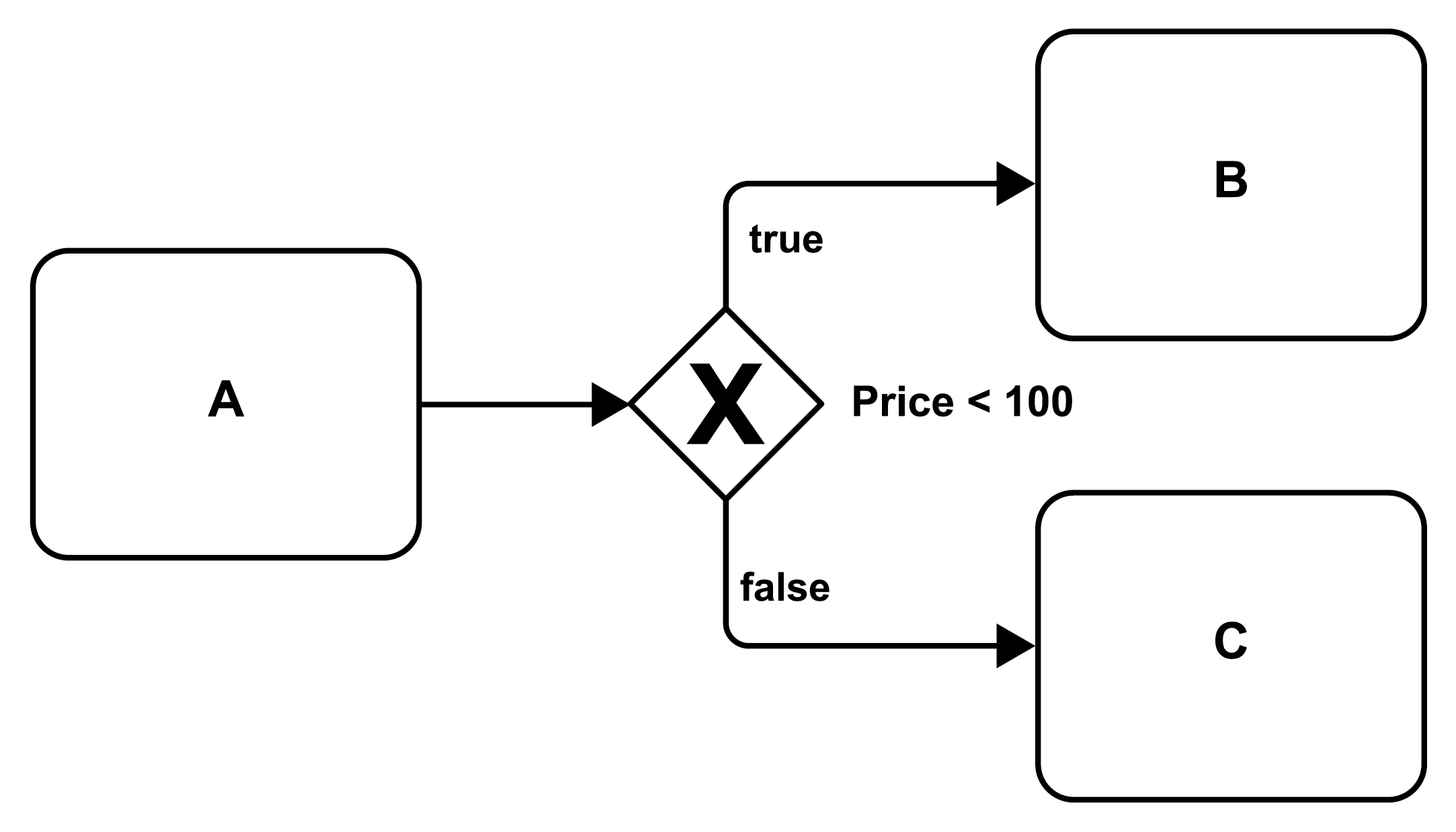
Figure 18: Alternative Execution via an Exclusive Split (XOR Split)

Between the unconditional parallel split (all paths are taken) in Figure 16 and the exclusive split (exactly one path will be taken) in the figure before, Figure 19 (compare the generic representation in Figure 3 part 4) shows an inclusive split. Any of the parallel paths originating from the gateway (i.e., the diamond decorated with a “○”) may be taken. In the figure, if the “duration is exceeded” activity B will be performed, and if also “credit card invalid” is true activity C will be performed in parallel. If only one condition is satisfied, the corresponding activity will be performed and the other path will not be followed. If none of the conditions evaluate to “true”, none of the paths will be followed, i.e., neither activity B nor activity C will take place. 

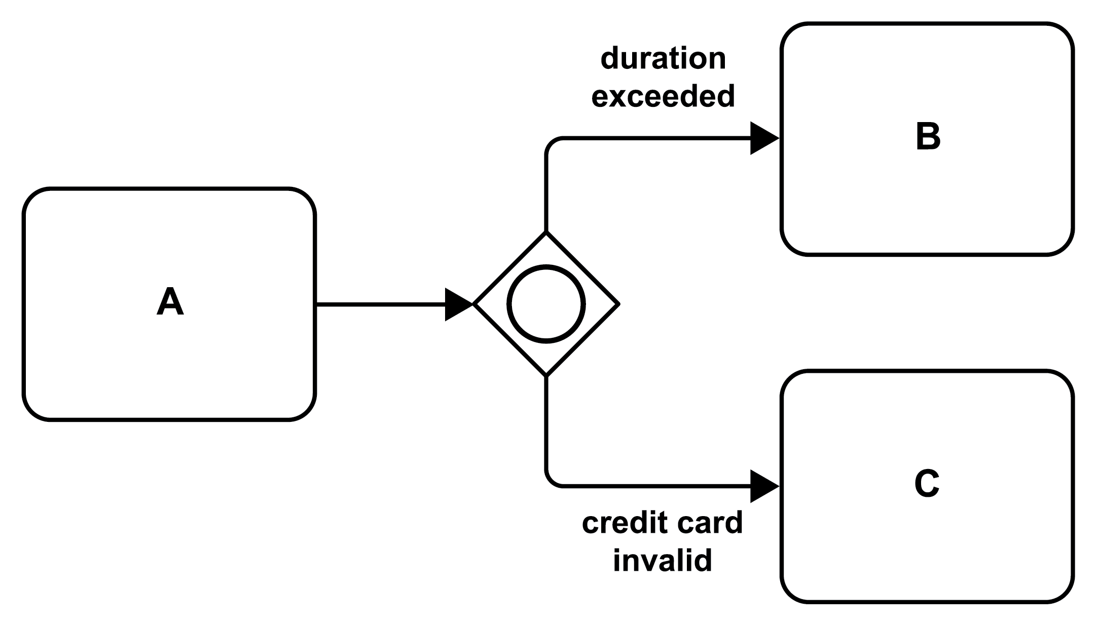
Figure 19: Conditional Parallel Branching via an Inclusive Split (IOR Split)

When the control flow is split it is often necessary (or at least good practice) to join the paths later on before continuing processing. Special care must be taken to join the control flow with the same kind of gateway that has been used to split the control flow. Otherwise, unexpected behavior may result (see [8]). Figure 20 (compare the generic representation in Figure 6 part 9 and part 10) shows two such well-formed fragments of diagrams of microflows: an exclusive join follows an exclusive split, and an inclusive join follows an inclusive split. 

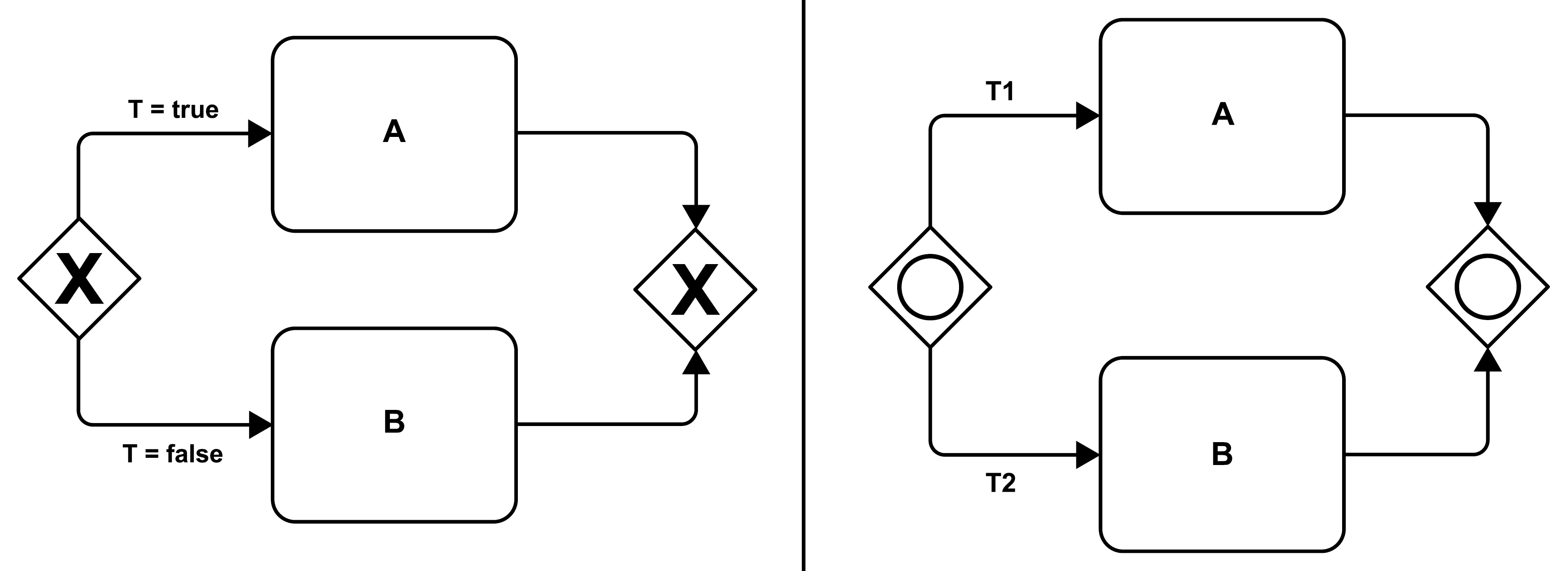
Figure 20: Matching Splits and Joins

BPMN also supports loops. In Figure 21 (compare the generic representation in Figure 4 part 5), an "until" loop is depicted: in part a, activities A and B are executed before the exclusive gateway checks whether "all agree"; if the answer is "no," both activities will be executed again. Otherwise, the loop is exited, and the control flow continues with the activity after the gateway. Part b illustrates the same loop using a special construct—a subflow (refer to Figure 5) included in a separate box, decorated with a directed circle indicating the loop behavior.

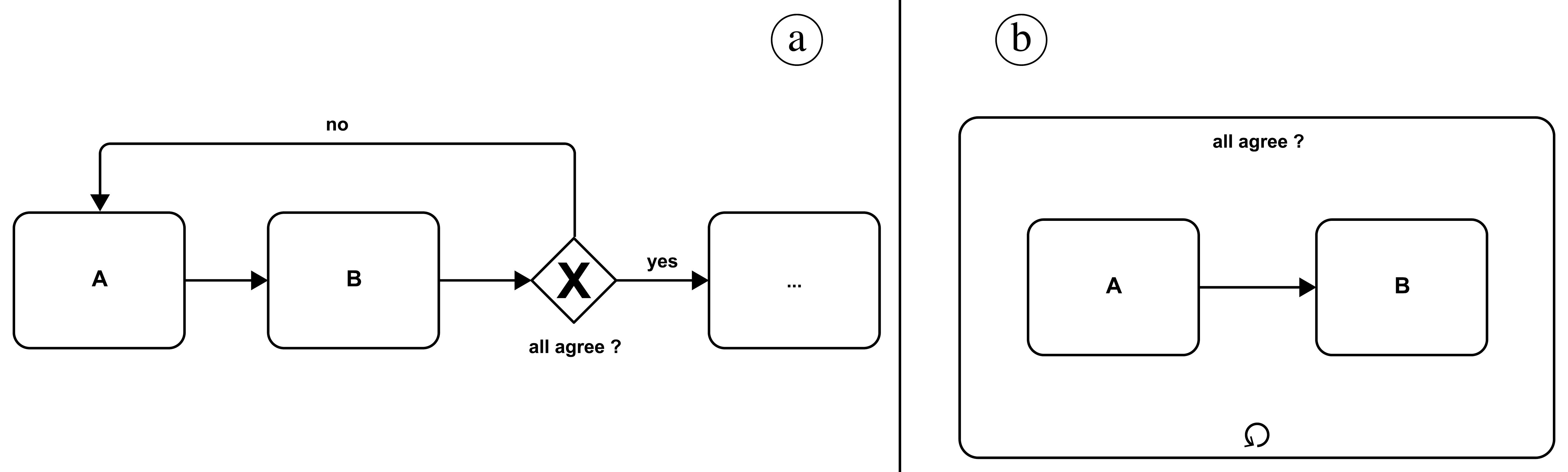
Figure 21: Do Until Loop

Similarly, a while loop is depicted in Figure 22 (compare the generic representation in Figure 4 part 6), if the condition “all agree” of the exclusive gateway is not satisfied, the loop is entered and activities A and B are performed sequentially. After that, the control flow returns to the gateway and the condition is checked again. In case the condition is met, the loop is left (or not even entered in the first place) and the control flow continues with the lower path. 

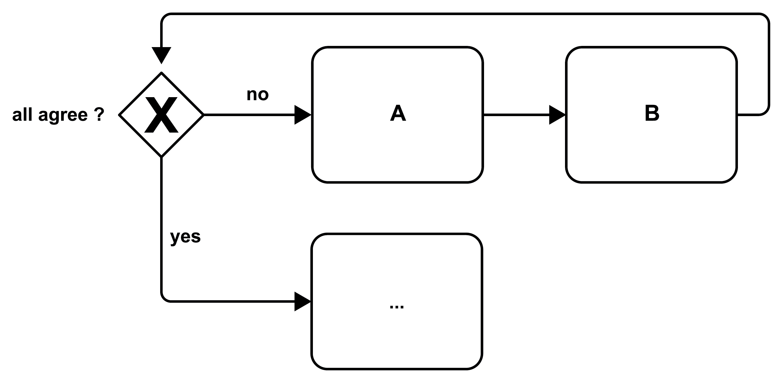
Figure 22: Do While Loop

Finally, BPMN supports subflows, i.e., microflows that implement an activity of the microflow proper. Figure 23 (compare the generic representation in Figure 5) includes activity S that is decorated by a “+” in the lower part of the activity icon. This “+” sign indicates that the activity contains a substructure, and this substructure is shown in the lower part of the figure as the implementation i(S) of the activity. In BPMN, an activity with an “+” decorator is referred to as a collapse subflow, while an activity with its substructure revealed (like also in Figure 21 part b) is called an expanded subflow. 

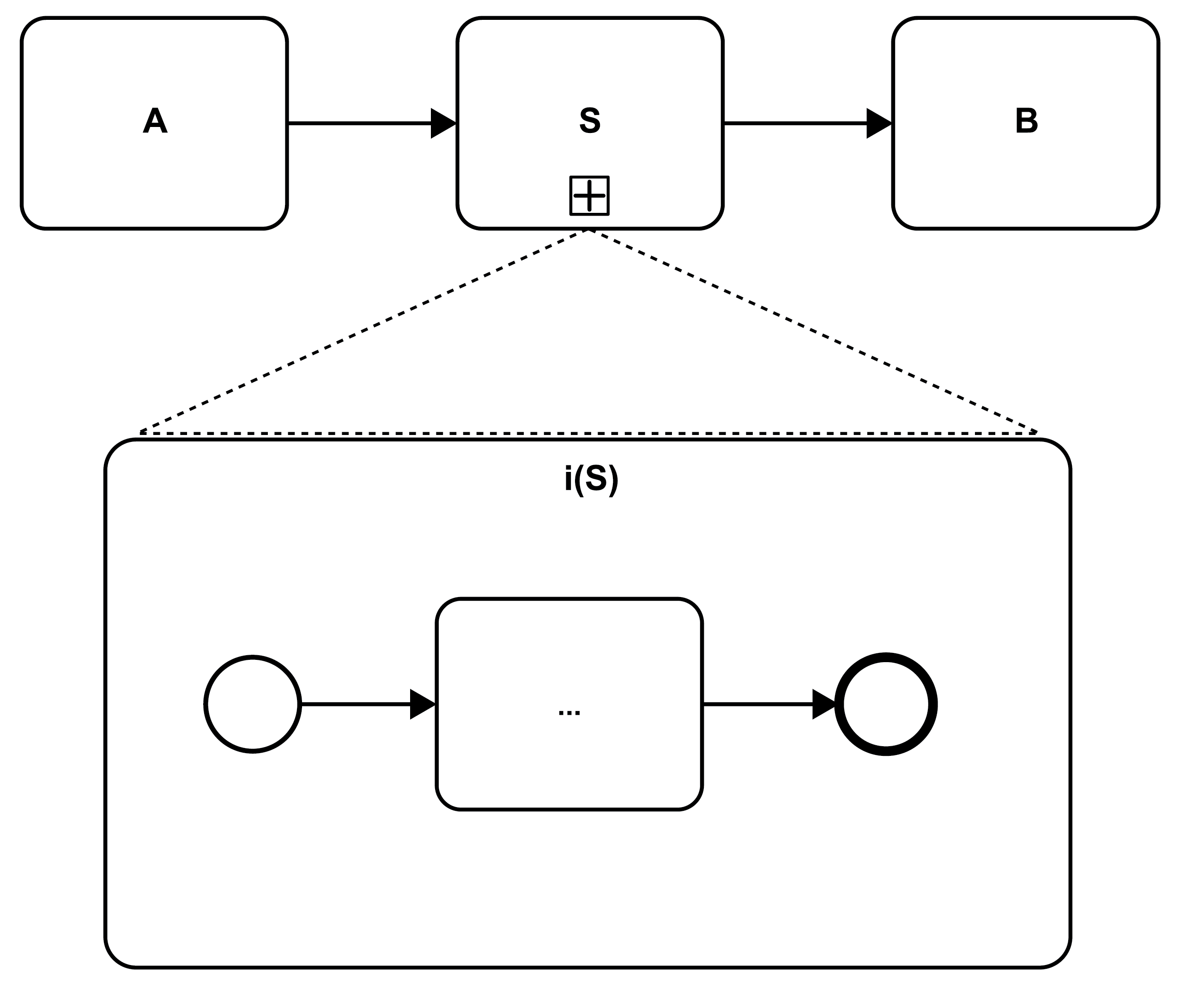
Figure 23: Subflows as Activity Implementations

3.3 Building Microflows with Ballerina

Ballerina is a programming language for integration, i.e., for building distributed applications by integrating existing functions [10]. It is grounded in the metaphor of sequence diagrams (see [16] section 17.8). In our context, Ballerina’s property of treating code and diagram equally is key, i.e., when writing code the corresponding sequence diagram is immediately depicted, and vice versa when drawing a sequence diagram the corresponding code is shown instantaneously. In the following, we sketch how Ballerina supports the key control flow features of microflows (see section 2.2). Ballerina also supports specifying data flows by realizing assignments as separate activities (see Figure 9) or by simply referring to variables from the signature of the activities. Since this does not involve separate constructs, data flows in Ballerina are not discussed.

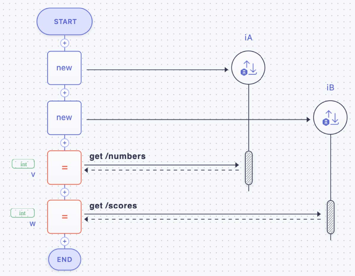Figure 24: A Sequence of Activities and Their Implementations

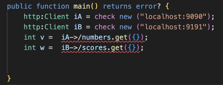
The figures in this section show on the left side (or lower part) a Ballerina code fragment and on the right side (or upper part) the corresponding rendering in a sequence diagram style generated by the Ballerina extension for Visual Studio Code [11]. In a nutshell, vertical lines (called lifelines) represent (in our context) the activity implementations that in turn may be realized as microflows (Figure 24). The leftmost lifeline is the microflow proper that is represented by the overall diagram. The lifeline of the microflow specifies its control flow. Also, the variables used to interact with the activity implementations are shown, building the variable pool of the microflow. The rounded lengthy rectangles in the lifeline of the activity implementations depict their execution. Horizontal lines represent request messages (solid lines) and response messages (dashed lines).

Figure 24 represents an unconditional execution (compare also the generic representation in Figure 3, part 1): two activity implementations iA and iB are shown (they are REST APIs as can be seen by the http:Client statements in code on the left side, or by the URLs decorating the request messages in the sequence diagram on the right side). The microflow is bracketed by the start and end symbols similar to Figure 15, and the microflow interacts with the APIs in an unconditional sequence. 

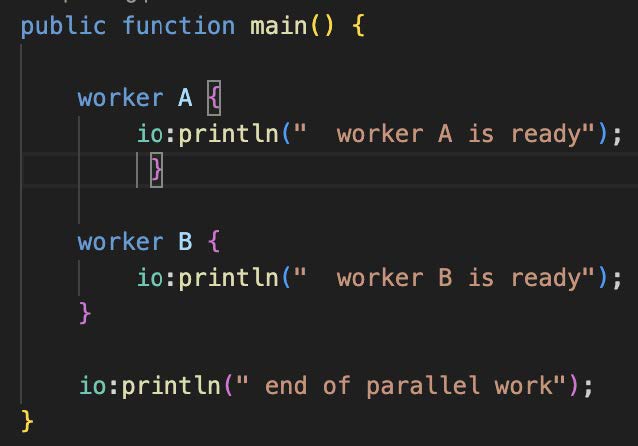
The next figure (Figure 25) gives an example of an AND split (compare Figure 16), i.e., an unconditional parallel execution of two activities (represented by lifelines A and B in the figure), followed sequentially by another activity (“println” bracketed by the start and end symbols of the microflow proper). The figure also shows decorations (like in Figure 2) of the activities indicating that all three activities are ”call” activities. Also, the control flow logic of activities A and B are depicted: both A and B print a text. 

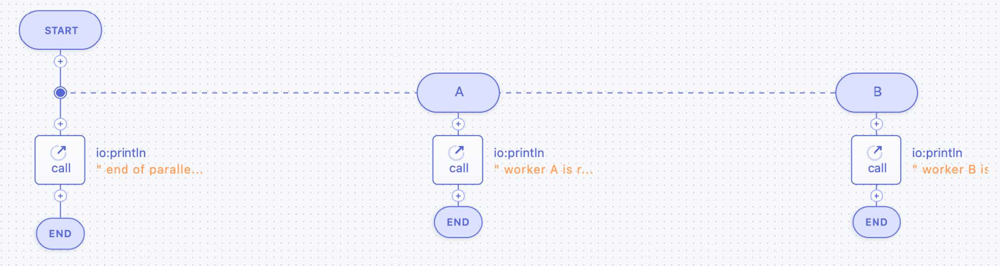Figure 25: Parallel Activities via an AND Split

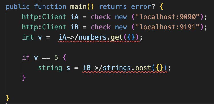
A conditional execution (compare also the generic representation in Figure 3 part 2) is exemplified in Figure 26: activity implementation iA is always executed, while activity implementation iB is executed in case the condition “v==5” is satisfied. 

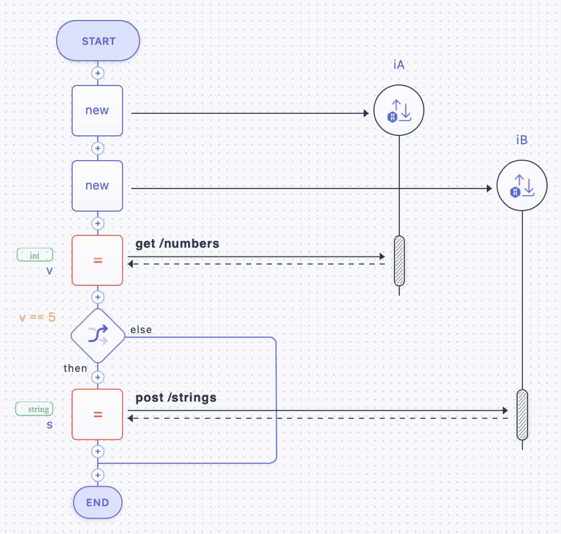Figure 26: Conditional Execution via an IF Statement

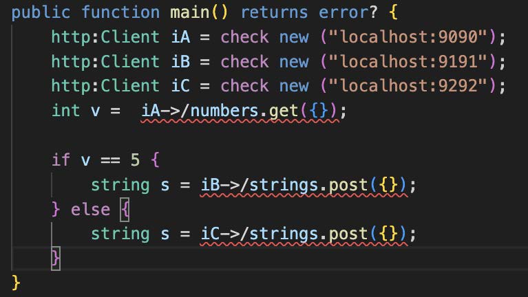
An exclusive split (compare Figure 18 and also Figure 3 part 3) is shown in Figure 27: three activities with implementations iA, iB, and iC are depicted. The first activity of the microflow retrieves some numbers from iA. Next, in case the condition “v==5” is satisfied, a string is posted to iB, otherwise, the string is posted to iC. 

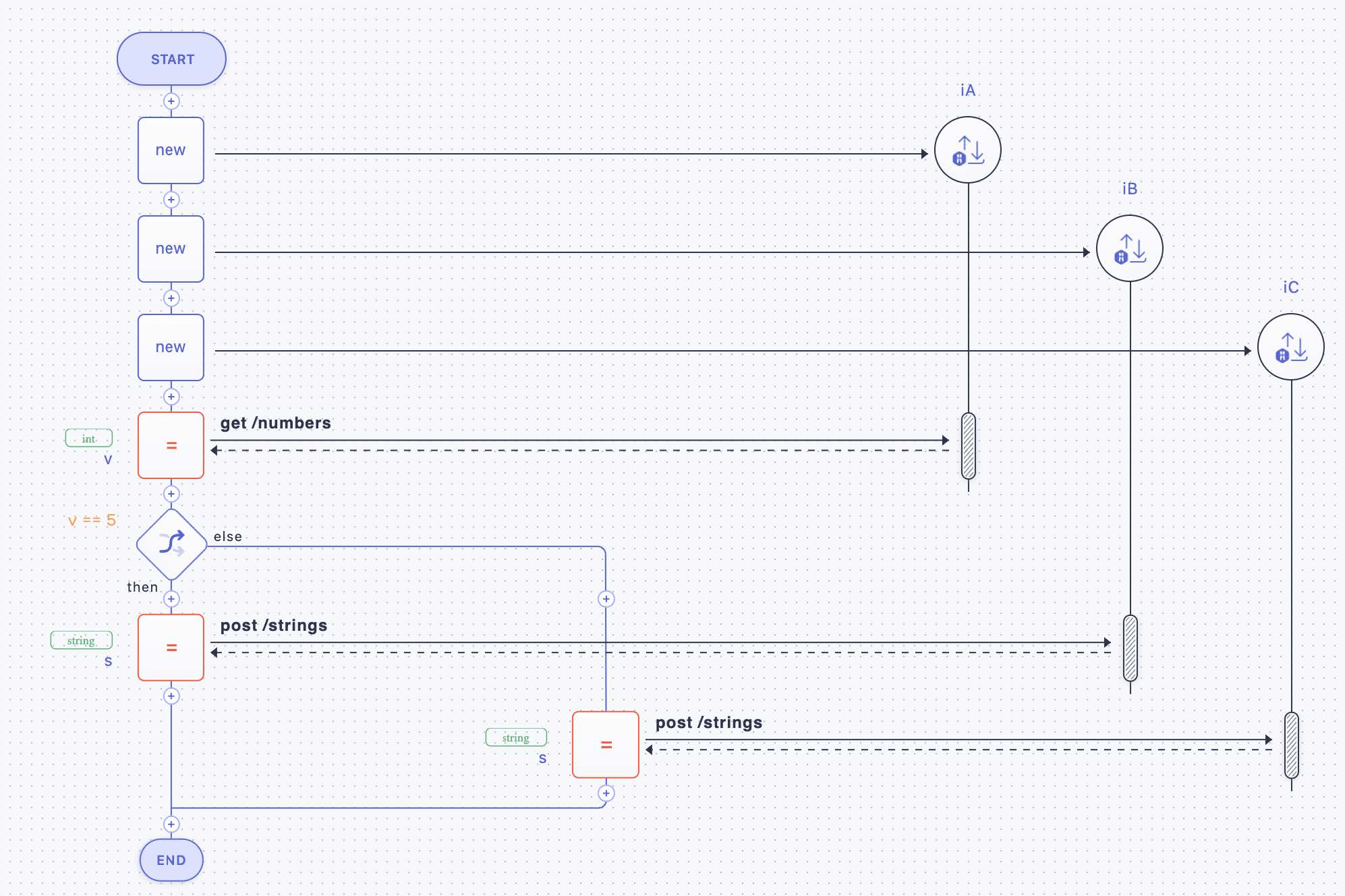Figure 27: Alternative Execution (Exclusive Split) via an IF-THEN-ELSE Statement

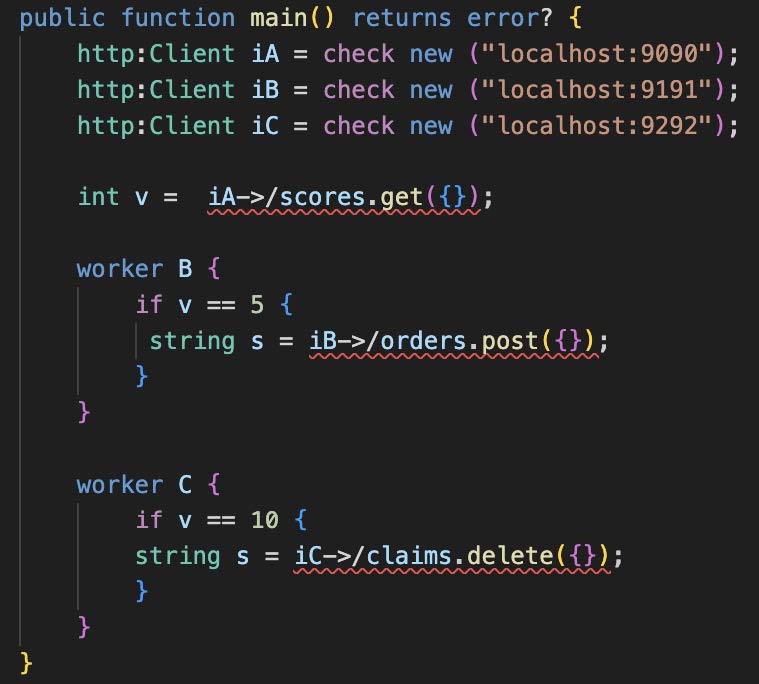
A conditional parallel branching, i.e., an IOR split (compare Figure 19 and also Figure 3 part 4), is depicted in Figure 28. Three activities iA, iB, and iC are shown. The interaction with iA is taken place by the microflow unconditionally. After that, iB and iC take place in case the conditions “v==5” and “v==10” are true, and orders are placed and claims are deleted. In case just “v==5” is true, just the orders are placed, and if only “v==10” is fulfilled, only the claims are deleted. If none of the conditions are true, the microflow is finished after the first activity. 

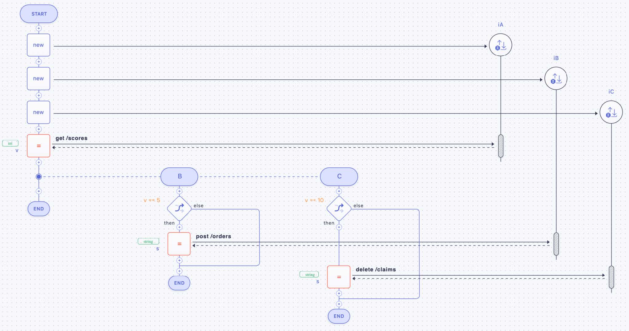Figure 28: Conditional Parallel Branching as IOR Split

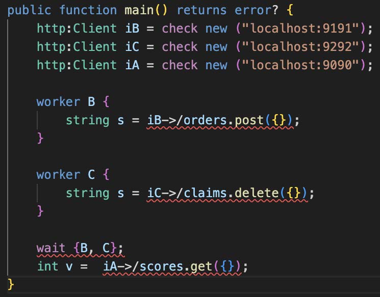
How parallel paths are joined is shown in Figure 29 (compare Figure 20 and also Figure 6 part 10): the two activities B and C are performed in parallel; activity B posts orders via activity implementation iB, C is deleting claims by means of activity implementation iC. The proper microflow (the leftmost lifeline in the figure) contains a “wait” activity; this activity completes as soon as both, activity B and activity C, are finished. After that, the microflow will interact with activity implementation iA by getting some scores.

Activities B and C are unconditionally running in parallel. Thus, the split of the control flow in two parallel paths is an AND split. Consequently, the corresponding join of the two paths represented by the “wait” activity in the microflow is an AND join. 

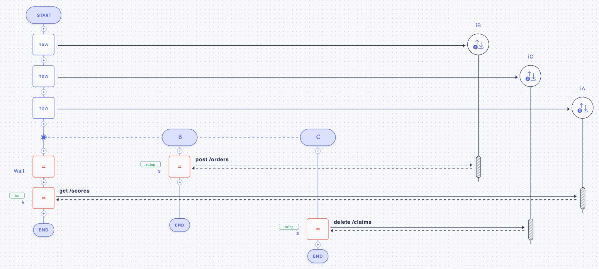Figure 29: An AND Join by Synchronizing via WAIT

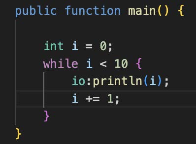
In Figure 30, a “while loop” is shown (compare Figure 22 and also Figure 4 part 6). The body of the loop is printing an integer and increases it. In the sequence diagram, this body is collapsed, indicated by the three dots. 

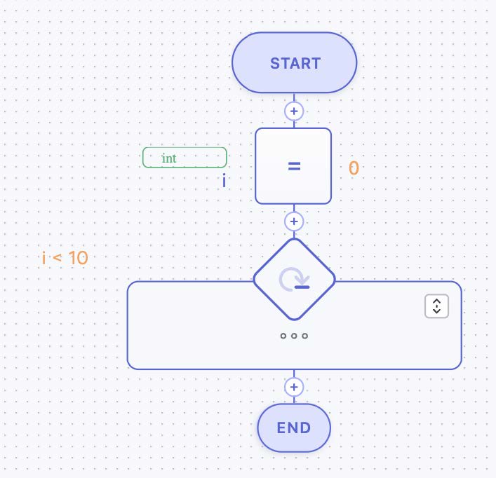Figure 30: WHILE Loop

4. Beyond Microflows 

Although microflows make use of many features well known from workflows, there are some significant differences between both. The first major difference is that workflow modeling supports considering the organizational structure of a company performing a business process. Another notable difference is native polyglottness of workflows in terms of activity implementations, which becomes irrelevant in an API-centric environment. Both aspects are discussed in section 4.1. 

Furthermore, workflows typically have significant quality of services that microflows lack, most notably interruptibility and robustness. Interruptibility implies that workflow technology is able to support long-running processes. And robustness materializes in various flavors of recoverability. Section 4.2 discusses these aspects.

4.1 Modeling Workflows

In sections 2.2 and 2.3 we discussed the control flow and data flow aspects of microflows that together are in the realm of the “what” dimension of workflow modeling (see section 3.1). Although microflows as defined cover the main constructs of control flow and data flow, there are several more such constructs that we left out of our definition like event handling. Such constructs are in fact supported by the standardized workflow languages BPMN and BPEL (see [15], [12]), and beyond these constructs, there are even more that are deemed to be desirable [7]. But all these additional constructs are not relevant in order to understand the essence of microflows, thus, we left them out. 

One fundamental difference between microflows and workflows from a modeling perspective is the aspect of organizational structures and activities performed by human beings in contrast to activities being automatically performed by programs (i.e., this is a difference in the “who” dimension discussed in section 3.1). This aspect is natively supported by BPMN and has been comprehensively standardized as an extension of BPEL [14]. As an example, Figure 31 depicts these aspects in the graphical syntax of BPMN. First, horizontal lines are shown that are referred to as swimlanes, and second a new decorator for user performed activities is shown. A swimlane represents organizational structures like departments or roles, for example. In the figure, the upper swimlane represents the “sales” department, the lower swimlane represents the “backoffice”. Within the swimlane representing the sales department, the activity “Inform Customer” is depicted; each activity placed into a swimlane must be performed by a representative of the corresponding organizational unit. The decorator of the activity in the “sales” swimlane specifies it as one to be performed by a human being, i.e., a member of the sales department is in charge to perform this activity. When this activity is completed, the control flow specifies that the “File Response” activity will be started, which is a service task that is automatically performed in the backoffice.

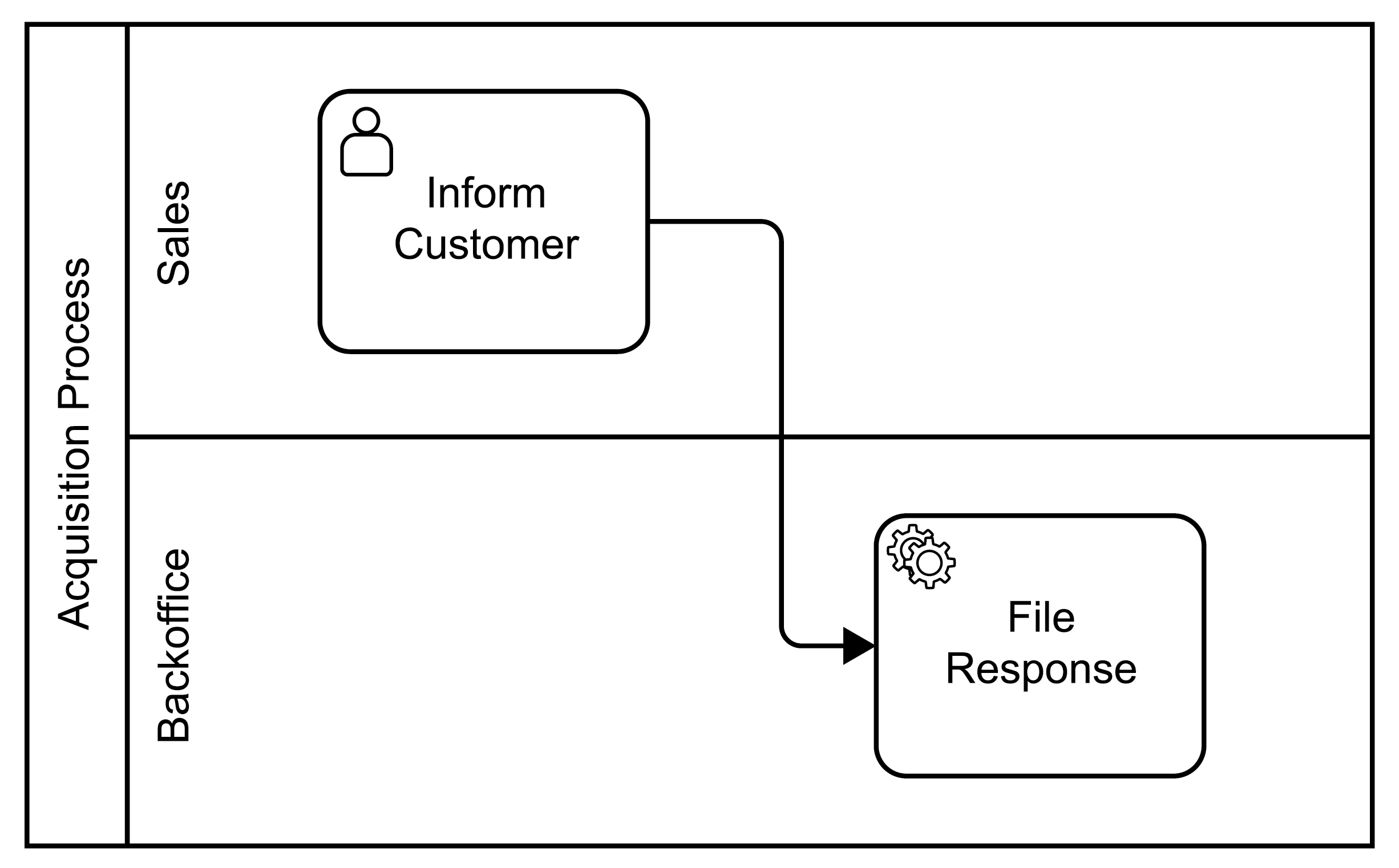
Figure 31: Sample Organizational Aspects

Thus, workflows support mixing activities performed by humans and activities that are automatically performed. Microflows support only the execution of activities that are automatically performed, i.e., not under the control of humans. Activating a user activity means to notify a human that a corresponding activity has to be performed. And a human finally decides when the implementation associated with the activity is actually executed, i.e., there is a delay between activating the activity and running its associated implementation [4]. 

Different people may use different implementations for a given user activity. For example, different users may prefer different email programs in order to inform a customer: thus, the association of an implementation is not a binary one between an activity and an implementation, but a ternary one between an activity, a user, and an implementation. In this sense, the binding of a user activity to an implementation is context-dependent (it depends on the user). In general, workflow technologies extend this context dependency beyond user activities to all activities and their implementations [4]: especially the implementation of a service activity may be chosen based on values of variables from the variable pool. For example, the automatically performed “File Response” activity may use an implementation storing the response in a log for negative responses, or a different implementation for storing the response in a database for positive responses. This dynamic binding capability is another difference between workflows and microflows, i.e., a difference within the “which” dimension of the W3-cube (see section 3.1). But dynamic binding of activity implementations is very rarely used in practice, and this is why this is not part of our definition of microflows. 

Finally, workflows are typically polyglott in the sense that they support interactions with activity implementations realized in a large spectrum of programming languages. Most workflow systems can directly interact properly with the corresponding environment of the implementation, transform parameters back and forth, and so on [4]. Today, most interactions are based on APIs, which hide implementation details of the program to interact with anyway. Thus, our definition of microflows ignores explicit polyglottness because it is a given based on the API technology being used. 

4.2 Operational Semantics

The very deep difference between a microflow and a workflow is in their operational semantics and their quality of services. In analogy to a program both a workflow and a microflow is a parallel and distributed program, i.e., its different steps (mainly the activities) may be executed at perhaps different locations and at the same time. This is because activity implementations may be deployed at different locations in the network and the microflow will interact with them via APIs, for example. Based on the parallel control flow constructs discussed in section 2.2 (and chapter 3), the implementations of parallel activities may be interacted with at the same time.

In addition to this, a workflow is also a persistent and transacted program. A workflow being a persistent program means that its variable pool as well as its overall execution state is stored persistently (at least as long as the program is running). Whenever the value of a variable of the pool is modified it is made persistent; whenever the state of the workflow is changed (e.g., when an activity is completed or activated, when a transaction condition has been evaluated, etc.), the corresponding information is persisted. 

A significant implication of this is that a workflow is interruptible. This is the key runtime feature that supports long-running business processes. When an activity is detected to be activated its implementation is not necessarily immediately started (the actual kind of behavior is controlled by corresponding parameters). Instead, the information that an activity “is ready” may be stored in a persistent store, and it may be selected at a later time for starting its implementation (see [4] section 10.5). This feature is especially useful for user activities allowing a person to work on an activity at suitable times. In contrast to this behavior, a microflow is not persistent, i.e., it is not interruptible, and it performs the implementation of an activity as soon as the activity is determined to be activated. As a consequence, a microflow executes “fast” by being performed in a “run and gun” manner.

4.3 Recoverability

Another significant consequence of persistence is forward recoverability of the overall workflow. When a workflow crashes (e.g., in case the environment performing a workflow fails) no formerly successfully finished work is lost. In a nutshell, during restart of the environment, the persistent state of the workflow is retrieved, activities that are ready to be performed are determined and processed (see [4] sections 10.5.7 and 10.5.8 for corresponding details as well as details about avoiding duplicate execution of activity implementations). 

Note, that a workflow without any user activities can be requested to be performed like a microflow. In this case, persistence is switched off, which results in a non-interruptible and non-forward recoverable behavior, i.e., this kind of workflow then behaves like a microflow. 

A workflow may not only be forward recoverable but also backward recoverable, i.e., it can undo collections of activities in case errors are detected. The collection of activities that share a joint outcome is referred to as a sphere (e.g., [4], [6]), i.e., the sphere is bracketing all activities that either must complete successfully or that must be undone in case they have been performed at the time an error is detected. 

In case all activities within a sphere are implemented by ACID transactions, the corresponding so-called atomic sphere ([4]) is expected to be run as a distributed transaction (see [6]). The corresponding behavior fits in a Java environment [13], for example. But often, activity implementations are not realized as ACID transactions. This is because activities of a workflow often manipulate resources that are not stored in a database (i.e., no transactions are supported by their underlying data stores), or the activities have impact on the real world (e.g., sending a letter), or the activities simply take such a long time that a transactional implementation will not work. 

But even if activities are implemented as transactions, executing collections of them as distributed transactions is prohibited especially in a microservice environment or in a cloud environment (see detailed arguments and discussion in [6]). In this case, each activity within a sphere must be associated with a compensation step that can undo whatever the activity performed (see [4] or [6] for details about compensation based recovery). Such so-called compensation spheres have been standardized in BPEL and BPMN ([12], [15]). If an error is encountered, the workflow will automatically perform the specified compensation steps of completed activities such that the compensation sphere will show the required all-or-nothing semantics. 

Microflows (in the sense of short-running, automatic workflows) can encompass atomic spheres or compensation spheres. But for this purpose, the environment offering microflows has to support the corresponding operational semantics. For example, BPMN supports compensation spheres while Ballerina supports atomic spheres. 

5. Concluding Remarks 

Microflows are an integration technology that allows the creation of new business functionality with little programming skills. This functionality is created based on a graphical metaphor supported by microflow environments. In this contribution, such a graphical metaphor has been defined in terms of control flow and data flow constructs at a product independent level to help a general understanding of the concept. Next, we have shown how microflows can be realized in BPMN as well as in Ballerina. While BPMN is geared towards the realization of business processes, Ballerina focuses on solving integration problems. Thus, the scope of BPMN and Ballerina is different but they intersect in support of our generic definition of a microflow. In order to contribute a deeper understanding of microflows, the key features of workflows that go beyond microflows have been discussed.

If pure integration problems have to be solved in a microservice context or in a cloud environment, Ballerina is a language to be considered. In case integration problems are at hand that are related to business processes, BPMN is a suitable language. 

6. References 

[1] G. Hohpe, B. Woolf: Enterprise Integration Patterns. Addison-Wesley (2004).

[2] M. Fowler: Patterns of Enterprise Application Architecture. Addison-Wesley (2003).

[3] F. Leymann et al.: REST API design guidelines. WSO2 (2016). 

[4] F. Leymann, D. Roller: Production workflow. Prentice Hall (2000).

[5] F. Leymann: BPEL vs. BPMN 2.0: Should You Care? In: Business Process Modeling Notation, Springer (2010).

[6] F. Leymann: Transactions in a microservices world. WSO2 (2023). 

[7] N. Russell, W.M.P. van der Aalst, A.H.M. ter Hofstede: Workflow Patterns.The MIT Press (2016).

[8] Bruce Silver: BPMN Method & Style. Cody- Cassidy Press (2009).

[9] S. Weerawarana, F. Curbera, F. Leymann, T. Storey, D. Ferguson: Web Services Platform Architecture. Prentice Hall (2005).

[10] https://ballerina.io/

[11] https://marketplace.visualstudio.com/items?itemName=WSO2.ballerina 

[12] http://docs.oasis-open.org/wsbpel/2.0/OS/wsbpel-v2.0-OS.html

[13] http://xml.coverpages.org/BPELJ-IBM-2004.pdf 

[14] http://docs.oasis-open.org/bpel4people/bpel4people-1.1.html 

[15] https://www.omg.org/spec/BPMN/2.0/PDF

[16] https://www.omg.org/spec/UML/2.5.1/PDF 

[17] https://camunda.com/download/modeler/

[18] https://camunda.com/download/platform-7/