Bayesian Learning for Machine Learning: Part I - Introduction to Bayesian Learning

In this blog, I will provide a basic introduction to Bayesian learning and explore topics such as frequentist statistics, the drawbacks of the frequentist method, Bayes’s theorem (introduced with an example), and the differences between the frequentist and Bayesian methods using the coin flip experiment as the example.

To begin with, let us try to answer this question: what is the frequentist method?

The Famous Coin Flip Experiment

When we flip a coin, there are two possible outcomes - heads or tails. Of course, there is a third rare possibility where the coin balances on its edge without falling onto either side, which we assume is not a possible outcome of the coin flip for our discussion. We conduct a series of coin flips and record our observations i.e. the number of the heads (or tails) observed for a certain number of coin flips. In this experiment, we are trying to determine the fairness of the coin, using the number of heads (or tails) that we observe.

Frequentist Statistics

Let us think about how we can determine the fairness of the coin using our observations in the above mentioned experiment. Once we have conducted a sufficient number of coin flip trials, we can determine the frequency or the probability of observing the heads (or tails). If we observed heads and tails with equal frequencies or the probability of observing heads (or tails) is $0.5$, then it can be established that the coin is a fair coin. Failing that, it is a biased coin. Let's denote $p$ as the probability of observing the heads. Consequently, as the quantity that $p$ deviates from $0.5$ indicates how biased the coin is, $p$ can be considered as the degree-of-fairness of the coin.

Testing whether a hypothesis is true or false by calculating the probability of an event in a prolonged experiment is known as frequentist statistics. As such, determining the fairness of a coin by using the probability of observing the heads is an example of frequentist statistics (a.k.a. frequentist approach).

Let us now further investigate the coin flip example using the frequentist approach. Since we have not intentionally altered the coin, it is reasonable to assume that we are using an unbiased coin for the experiment. When we flip the coin $10$ times, we observe the heads $6$ times. Therefore, the $p$ is $0.6$ (note that $p$ is the number of heads observed over the number of total coin flips). Hence, according to frequencies statistics, the coin is a biased coin — which opposes our assumption of a fair coin. Perhaps one of your friends who is more skeptical than you extends this experiment to $100$ trails using the same coin. Then she observes heads $55$ times, which results in a different $p$ with $0.55$. Even though the new value for $p$ does not change our previous conclusion (i.e. that the coin is biased), this observation raises several questions:

• How confident are we of $p$ being $0.6$?
• How confident are of $p$ being $0.55$?
• Which of these values is the accurate estimation of $p$?
• Will $p$ continue to change when we further increase the number of coin flip trails?

We cannot find out the exact answers to the first three questions using frequentist statistics. We may assume that true value of $p$ is closer to $0.55$ than $0.6$ because the former is computed using observations from a considerable number of trials compared to what we used to compute the latter. Yet there is no way of confirming that hypothesis. However, if we further increase the number of trials, we may get a different probability from both of the above values for observing the heads and eventually, we may even discover that the coin is a fair coin.

Number of coin flips	Number of heads	Probability of observing heads
10	6	0.6
50	29	0.58
100	55	0.55
200	94	0.47
500	245	0.49

Table 1 - Coin flip experiment results when increasing the number of trials

Table 1 presents some of the possible outcomes of a hypothetical coin flip experiment when we are increasing the number of trials. The fairness ($p$) of the coin changes when increasing the number of coin-flips in this experiment. Our confidence of estimated $p$ may also increase when increasing the number of coin-flips, yet the frequentist statistic does not facilitate any indication of the confidence of the estimated $p$ value. We can attempt to understand the importance of such a confident measure by studying the following cases:

• An experiment with an infinite number of trials guarantees $p$ with absolute accuracy (100% confidence). Yet, it is not practical to conduct an experiment with an infinite number of trials and we should stop the experiment after a sufficiently large number of trials. However, deciding the value of this sufficient number of trials is a challenge when using frequentist statistics.
• If we can determine the confidence of the estimated $p$ value or the inferred conclusion, in a situation where the number of trials are limited, this will allow us to decide whether to accept the conclusion or to extend the experiment with more trials until it achieves sufficient confidence.

Moreover, we may have valuable insights or prior beliefs (for example, coins are usually fair and the coin used is not made biased intentionally, therefore $p\approx0.5$) that describes the value of $p$ . Embedding that information can significantly improve the accuracy of the final conclusion. Such beliefs play a significant role in shaping the outcome of a hypothesis test especially when we have limited data. However, with frequentist statistics, it is not possible to incorporate such beliefs or past experience to increase the accuracy of the hypothesis test.

Some Terms to Understand

Before delving into Bayesian learning, it is essential to understand the definition of some terminologies used. I will not provide lengthy explanations of the mathematical definition since there is a lot of widely available content that you can use to understand these concepts.

• Random variable (Stochastic variable) - In statistics, the random variable is a variable whose possible values are a result of a random event. Therefore, each possible value of a random variable has some probability attached to it to represent the likelihood of those values.
• Probability distribution - The function that defines the probability of different outcomes/values of a random variable. The continuous probability distributions are described using probability density functions whereas discrete probability distributions can be represented using probability mass functions.
• Conditional probability - This is a measure of probability $P(A|B)$ of an event A given that another event B has occurred.
• Joint probability distribution

Introduction to Bayesian Learning

Imagine a situation where your friend gives you a new coin and asks you the fairness of the coin (or the probability of observing heads) without even flipping the coin once. In fact, you are also aware that your friend has not made the coin biased. In general, you have seen that coins are fair, thus you expect the probability of observing heads is $0.5$. In the absence of any such observations, you assert the fairness of the coin only using your past experiences or observations with coins.

Suppose that you are allowed to flip the coin $10$ times in order to determine the fairness of the coin. Your observations from the experiment will fall under one of the following cases:

• Case 1: observing $5$ heads and $5$ tails.
• Case 2: observing $h$ heads and $10-h$ tails, where $h\neq 10-h$.

If case 1 is observed, you are now more certain that the coin is a fair coin, and you will decide that the probability of observing heads is $0.5$ with more confidence. If case 2 is observed you can either:

1. Neglect your prior beliefs since now you have new data, decide the probability of observing heads is $h/10$ by solely depending on recent observations.
2. Adjust your belief accordingly to the value of $h$ that you have just observed, and decide the probability of observing heads using your recent observations.

The first method suggests that we use the frequentist method, where we omit our beliefs when making decisions. However, the second method seems to be more convenient because $10$ coins are insufficient to determine the fairness of a coin. Therefore, we can make better decisions by combining our recent observations and beliefs that we have gained through our past experiences. It is this thinking model which uses our most recent observations together with our beliefs or inclination for critical thinking that is known as Bayesian thinking.

Moreover, assume that your friend allows you to conduct another $10$ coin flips. Then we can use these new observations to further update our beliefs. As we gain more data, we can incrementally update our beliefs increasing the certainty of our conclusions. This is known as incremental learning, where you update your knowledge incrementally with new evidence.

Bayesian learning comes into play on such occasions, where we are unable to use frequentist statistics due to the drawbacks that we have discussed above. We can use Bayesian learning to address all these drawbacks and even with additional capabilities (such as incremental updates of the posterior) when testing a hypothesis to estimate unknown parameters of a machine learning models. Bayesian learning uses Bayes’ theorem to determine the conditional probability of a hypotheses given some evidence or observations.

Bayes’ Theorem

Bayes’ theorem describes how the conditional probability of an event or a hypothesis can be computed using evidence and prior knowledge. It is similar to concluding that our code has no bugs given the evidence that it has passed all the test cases, including our prior belief that we have rarely observed any bugs in our code. However, this intuition goes beyond that simple hypothesis test where there are multiple events or hypotheses involved (let us not worry about this for the moment).

The Bayes’ theorem is given by:

$$P(\theta|X) = \frac{P(X|\theta)P(\theta)}{P(X)}$$

I will now explain each term in Bayes’ theorem using the above example. Consider the hypothesis that there are no bugs in our code. $\theta$ and $X$ denote that our code is bug free and passes all the test cases respectively.

• $P(\theta)$ - Prior Probability is the probability of the hypothesis $\theta$ being true before applying the Bayes’ theorem. Prior represents the beliefs that we have gained through past experience, which refers to either common sense or an outcome of Bayes’ theorem for some past observations.For the example given, prior probability denotes the probability of observing no bugs in our code. However, since this is the first time we are applying Bayes’ theorem, we have to decide the priors using other means (otherwise we could use the previous posterior as the new prior). Let us assume that it is very unlikely to find bugs in our code because rarely have we observed bugs in our code in the past. With our past experience of observing fewer bugs in our code, we can assign our prior $P(\theta)$ with a higher probability. However, for now, let us assume that $P(\theta) = p$.
• $P(X|\theta)$ - Likelihood is the conditional probability of the evidence given a hypothesis. The likelihood is mainly related to our observations or the data we have. If it is given that our code is bug free, then the probability of our code passing all test cases is given by the likelihood. Assuming we have implemented these test cases correctly, if no bug is presented in our code, then it should pass all the test cases. Therefore, the likelihood $P(X|\theta) = 1$.
• $P(X)$ - Evidence term denotes the probability of evidence or data. This can be expressed as a summation (or integral) of the probabilities of all possible hypotheses weighted by the likelihood of the same.

  Therefore, we can write $P(X)$ as:

  $$P(X) = \sum_{\theta\in\Theta}P(X|\theta)P(\theta)$$ , where $\Theta$ is the set of all the hypotheses.

  For the continuous $\theta$ we write $P(X)$ as an integration:

  $$P(X) =\int_{\theta}P(X|\theta)P(\theta)d\theta$$

  In the above example there are only two possible hypotheses, 1) observing no bugs in our code or 2) observing a bug in our code. Therefore we can denotes evidence as follows:

  $$P(X) = P(X|\theta)P(\theta)+ P(X|\neg\theta)P(\neg\theta)$$

  $\neg\theta$ denotes observing a bug in our code. Therefore, $P(X|\neg\theta)$ is the conditional probability of passing all the tests even when there are bugs present in our code. This term depends on the test coverage of the test cases. Even though we do not know the value of this term without proper measurements, in order to continue this discussion let us assume that $P(X|\neg\theta) = 0.5$. Accordingly,

  $$P(X) = 1 \times p + 0.5 \times (1-p) = 0.5(1 + p)$$

• $P(\theta|X)$ - Posteriori probability denotes the conditional probability of the hypothesis $\theta$ after observing the evidence $X$. This is the probability of observing no bugs in our code given that it passes all the test cases. Since we now know the values for the other three terms in the Bayes’ theorem, we can calculate the posterior probability using the following formula:

  $$P(\theta|X) = \frac {1 \times p}{0.5(1 + p)}$$

  We can also calculate the probability of observing a bug, given that our code passes all the test cases $P(\neg\theta|X)$ .

  \begin{align}P(\neg\theta|X) &= \frac{P(X|\neg\theta).P(\neg\theta)}{P(X)} \\ &= \frac{0.5 \times (1-p)}{ 0.5 \times (1 + p)} \\ &= \frac{(1-p)}{(1 + p)}\end{align}

  We now know both conditional probabilities of observing a bug in the code and not observing the bug in the code. Yet how are we going to confirm the valid hypothesis using these posterior probabilities?

Maximum a Posteriori (MAP)

We can use MAP to determine the valid hypothesis from a set of hypotheses. According to MAP, the hypothesis that has the maximum posterior probability is considered as the valid hypothesis. Therefore, we can express the hypothesis $\theta_{MAP}$ that is concluded using MAP as follows:

\begin{align}\theta_{MAP} &= argmax_\theta P(\theta_i|X) \\ &= argmax_\theta \Bigg( \frac{P(X|\theta_i)P(\theta_i)}{P(X)}\Bigg)\end{align}

The $argmax_\theta$ operator estimates the event or hypothesis $\theta_i$ that maximizes the posterior probability $P(\theta_i|X)$. Let us apply MAP to the above example in order to determine the true hypothesis:

$$\theta_{MAP} = argmax_\theta \Big\{ \theta :P(\theta|X)= \frac{p} { 0.5(1 + p)}, \neg\theta : P(\neg\theta|X) = \frac{(1-p)}{ (1 + p) }\Big\}$$

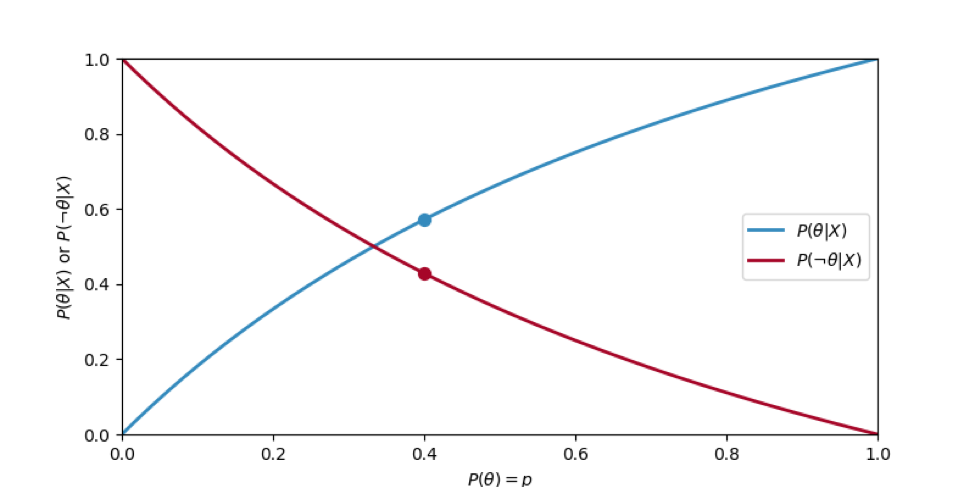
Figure 1 - $P(\theta|X)$ and $P(\neg\theta|X)$ when changing the $P(\theta) = p$

Figure 1 illustrates how the posterior probabilities of possible hypotheses change with the value of prior probability. Unlike frequentist statistics where our belief or past experience had no influence on the concluded hypothesis, Bayesian learning is capable of incorporating our belief to improve the accuracy of predictions. Assuming that we have fairly good programmers and therefore the probability of observing a bug is $P(\theta) = 0.4$ , then we find the $\theta_{MAP}$:

\begin{align}MAP &= argmax_\theta \Big\{ \theta:P(|X) = \frac{0.4 }{ 0.5 (1 + 0.4)}, \neg\theta : P(\neg\theta|X) = \frac{0.5(1-0.4)} {0.5 (1 + 0.4)} \Big\} \\&= argmax_\theta \Big\{\theta : P(\theta|X)=0.57, \neg\theta:P(\neg\theta|X) = 0.43 \Big\} \\&= \theta \implies \text{No bugs present in our code} \end{align}

However, $P(X)$ is independent of $\theta$, and thus $P(X)$ is same for all the events or hypotheses. Therefore, we can simplify the $\theta_{MAP}$ estimation, without the denominator of each posterior computation as shown below:

$$\theta_{MAP} = argmax_\theta \Big( P(X|\theta_i)P(\theta_i)\Big)$$

Notice that MAP estimation algorithms do not compute posterior probability of each hypothesis to decide which is the most probable hypothesis. Assuming that our hypothesis space is continuous (i.e. fairness of the coin encoded as probability of observing heads, coefficient of a regression model, etc.), where endless possible hypotheses are present even in the smallest range that the human mind can think of, or for even a discrete hypothesis space with a large number of possible outcomes for an event, we do not need to find the posterior of each hypothesis in order to decide which is the most probable hypothesis. Therefore, the practical implementation of MAP estimation algorithms use approximation techniques, which are capable of finding the most probable hypothesis without computing posteriors or only by computing some of them.

Using the Bayesian theorem, we can now incorporate our belief as the prior probability, which was not possible when we used frequentist statistics. However, we still have the problem of deciding a sufficiently large number of trials or attaching a confidence to the concluded hypothesis. This is because the above example was solely designed to introduce the Bayesian theorem and each of its terms. Let us now gain a better understanding of Bayesian learning to learn about the full potential of Bayes’ theorem.

Bayesian Learning

So far we have discussed Bayes’ theorem and gained an understanding of how we can apply Bayes’ theorem to test our hypotheses. However, when using single point estimation techniques such as MAP, we will not be able to exploit the full potential of Bayes’ theorem. I used single values (e.g. $P(X|\theta) = 1$ and $P(\theta) = p$ etc ) to explain each term in Bayes’ theorem to simplify my explanation of Bayes’ theorem. With Bayesian learning, we are dealing with random variables that have probability distributions. Let us try to understand why using exact point estimations can be misleading in probabilistic concepts.

Consider the prior probability of not observing a bug in our code in the above example. We defined that the event of not observing bug is $\theta$ and the probability of producing a bug free code $P(\theta)$ was taken as $p$. However, the event $\theta$ can actually take two values - either $true$ or $false$ - corresponding to not observing a bug or observing a bug respectively. Therefore, observing a bug or not observing a bug are not two separate events, they are two possible outcomes for the same event $\theta$. Since all possible values of $\theta$ are a result of a random event, we can consider $\theta$ as a random variable. Therefore, $P(\theta)$ is not a single probability value, rather it is a discrete probability distribution that can be described using a probability mass function.

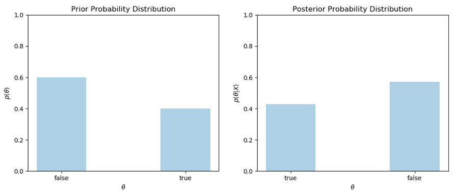
Figure 2 - Prior distribution $P(\theta)$ and Posterior distribution $P(\theta|X)$ as a probability distribution

Figure 2 illustrates the probability distribution $P(\theta)$ assuming that $p = 0.4$. Therefore, $P(\theta)$ can be either $0.4$ or $0.6$ which is decided by the value of $\theta$ (i.e. whether $\theta$ is $true$ of $false$). If we apply the Bayesian rule using the above prior, then we can find a posterior distribution$P(\theta|X)$ instead a single point estimation for that. Figure 2 also shows the resulting posterior distribution. You may recall that we have already seen the values of the above posterior distribution and found that $P(\theta = true|X) = 0.57$ and $P(\theta=false|X) = 0.43 $. Notice that I used $\theta = false$ instead of $\neg\theta$. This is because we do not consider $\theta$ and $\neg\theta$ as two separate events — they are the outcomes of the single event $\theta$. Even though MAP only decides which is the most likely outcome, when we are using the probability distributions with Bayes’ theorem, we always find the posterior probability of each possible outcome for an event.

You may wonder why we are interested in looking for full posterior distributions instead of looking for the most probable outcome or hypothesis. If we use the MAP estimation, we would discover that the most probable hypothesis is discovering no bugs in our code given that it has passed all the test cases. Remember that MAP does not compute the posterior of all hypotheses, instead it estimates the maximum probable hypothesis through approximation techniques. In fact, MAP estimation algorithms are only interested in finding the mode of full posterior probability distributions. However, if we compare the probabilities of $P(\theta = true|X)$ and $P(\theta = false|X)$, then we can observe that the difference between these probabilities is only $0.14$. Hence, there is a good chance of observing a bug in our code even though it passes all the test cases. According to the posterior distribution, there is a higher probability of our code being bug free, yet we are uncertain whether or not we can conclude our code is bug free simply because it passes all the current test cases. We can now observe that due to this uncertainty we are required to either improve the model by feeding more data or extend the coverage of test cases in order to reduce the probability of passing test cases when the code has bugs. We can perform such analyses incorporating the uncertainty or confidence of the estimated posterior probability of events only if the full posterior distribution is computed instead of using single point estimations. To further understand the potential of these posterior distributions, let us now discuss the coin flip example in the context of Bayesian learning.

I will define the fairness of the coin as $\theta$. We can use the probability of observing heads to interpret the fairness of the coin by defining $\theta = P(heads)$. Hence, $\theta = 0.5$ for a fair coin and deviations of $\theta$ from $0.5$ can be used to measure the bias of the coin. Since the fairness of the coin is a random event, $\theta$ is a continuous random variable. As such, the prior, likelihood, and posterior are continuous random variables that are described using probability density functions.

Let us now attempt to determine the probability density functions for each random variable in order to describe their probability distributions.

Binomial Likelihood

The likelihood for the coin flip experiment is given by the probability of observing heads out of all the coin flips given the fairness of the coin. As we have defined the fairness of the coins ($\theta$) using the probability of observing heads for each coin flip, we can define the probability of observing heads or tails given the fairness of the coin $P(y|\theta)$ where $y = 1$ for observing heads and $y = 0$ for observing tails. Accordingly:

\begin{align} P(y=1|\theta) &= \theta \\ P(y=0|\theta) &= (1-\theta) \end{align}

Now that we have defined two conditional probabilities for each outcome above, let us now try to find the $P(Y=y|\theta)$ joint probability of observing heads or tails:

$$ P(Y=y|\theta) = \begin{cases} \theta, \text{ if } y =1 \\1-\theta, \text{ otherwise } \end{cases} $$

Note that $y$ can only take either $0$ or $1$, and $\theta$ will lie within the range of $[0,1]$. We can rewrite the above expression in a single expression as follows:

$$P(Y=y|\theta) = \theta^y \times (1-\theta)^{1-y}$$

The above equation represents the likelihood of a single test coin flip experiment. Interestingly, the likelihood function of the single coin flip experiment is similar to the Bernoulli probability distribution. The Bernoulli distribution is the probability distribution of a single trial experiment with only two opposite outcomes. As the Bernoulli probability distribution is the simplification of Binomial probability distribution for a single trail, we can represent the likelihood of a coin flip experiment that we observe $k$ number of heads out of $N$ number of trials as a Binomial probability distribution as shown below:

$$P(k, N |\theta )={N \choose k} \theta^k(1-\theta)^{N-k} $$

Beta Prior Distribution

The prior distribution is used to represent our belief about the hypothesis based on our past experiences. We can choose any distribution for the prior, if it represents our belief regarding the fairness of the coin. For this example, we use Beta distribution to represent the prior probability distribution as follows:

$$P(\theta)=\frac{\theta^{\alpha-1}(1-\theta)^{\beta-1}}{B(\alpha,\beta)}$$

In this instance, $\alpha$ and $\beta$ are the shape parameters. We can use these parameters to change the shape of the beta distribution. $B(\alpha, \beta)$ is the Beta function. Beta function acts as the normalizing constant of the Beta distribution.

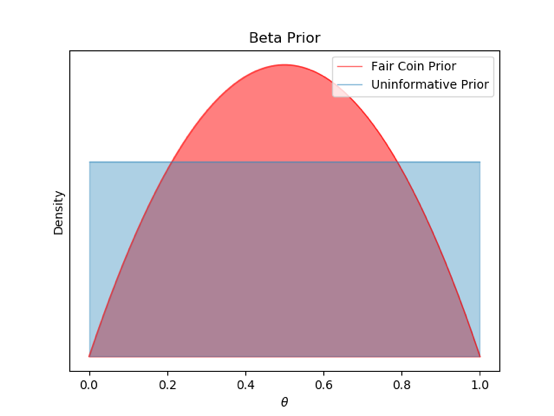
Figure 3 - Beta distribution for for a fair coin prior and uninformative prior

Reasons for choosing the beta distribution as the prior as follows:

• If the posterior distribution has the same family as the prior distribution then those distributions are called as conjugate distributions, and the prior is called the conjugate prior. Beta prior acts as a conjugate prior to Binomial likelihood. If we use a Beta distribution to represent our belief, then the resulting posterior distribution will also be a beta distribution. When we observe new data, then this posterior can be used as the new prior to compute the new posterior. Therefore, we can incrementally update the prior whenever new data is available avoiding many complex computations from Bayes’ theorem — the posterior can be derived by altering the shape parameters of the conjugate priors accordingly. We will discuss such a derivation of the posterior distribution in the section on posterior distribution.
• Beta distribution has a normalizing constant, thus it is always distributed between $0$ and $1$. Therefore we are not required to compute the denominator of the Bayes’ theorem to normalize the posterior probability distribution — Beta distribution can be directly used as a probability density function of $\theta$ (recall that $\theta$ is also a probability and therefore it takes values between $0$ and $1$).
• We can easily represent our prior belief regarding the fairness of the coin using beta function. As shown in Figure 3, we can represent our belief in a fair coin with a distribution that has the highest density around $\theta=0.5$. However, it should be noted that even though we can use our belief to determine the peak of the distribution, deciding on a suitable variance for the distribution can be difficult.
• If one has no belief or past experience, then we can use Beta distribution to represent an uninformative prior (Figure 3). When we are unable to decide the prior distribution due to lack of past experience, we can use the uninformative prior with minimal influence on the posterior. An uninformative prior can be generated by setting the shape parameters of Beta distribution $\alpha=\beta=1$.

Posterior Distribution

I previously mentioned that Beta is a conjugate prior and therefore the posterior distribution should also be a Beta distribution. Let us now try to derive the posterior distribution analytically using the Binomial likelihood and the Beta prior.

First of all, consider the product of Binomial likelihood and Beta prior:

\begin{align} P(X|\theta) \times P(\theta) &= P(N, k|\theta) \times P(\theta) \\ &={N \choose k} \theta^k(1-\theta)^{N-k} \times \frac{\theta^{\alpha-1}(1-\theta)^{\beta-1}}{B(\alpha,\beta)} \\ &=\frac{N \choose k}{B(\alpha,\beta)} \times \theta^{(k+\alpha) - 1} (1-\theta)^{(N+\beta-k)-1} \\ \end{align}

The posterior distribution of $\theta$ given $N$ and $k$ is:

\begin{align} P(\theta|N, k) &= \frac{P(N, k|\theta) \times P(\theta)}{P(N, k)} \\ &= \frac{N \choose k}{B(\alpha,\beta)\times P(N, k)} \times \theta^{(k+\alpha) - 1} (1-\theta)^{(N+\beta-k)-1} \\ \end{align}

Let $\alpha_{new}=k+\alpha$ and $\beta_{new}=(N+\beta-k)$:

$$ P(\theta|N, k) = \frac{N \choose k}{B(\alpha,\beta)\times P(N, k)} \times \theta^{\alpha_{new} - 1} (1-\theta)^{\beta_{new}-1} \\ $$

If we consider $\alpha_{new}$ and $\beta_{new}$ to be new shape parameters of a Beta distribution, then the above expression we get for posterior distribution $P(\theta|N, k)$ can be defined as a new Beta distribution with a normalising factor $B(\alpha_{new}, \beta_{new})$ only if:

$$ B(\alpha_{new}, \beta_{new}) = \frac{N \choose k}{B(\alpha,\beta)\times P(N, k)} $$

However, we know for a fact that both posterior probability distribution and the Beta distribution are in the range of $0$ and $1$. In order for $P(\theta|N, k)$ to be distributed in the range of 0 and 1, the above relationship should hold true. As such, we can rewrite the posterior probability of the coin flip example as a Beta distribution with new shape parameters $\alpha_{new}=k+\alpha$ and $\beta_{new}=(N+\beta-k)$:

$$ P(\theta|N, k) = \frac{\theta^{\alpha_{new} - 1} (1-\theta)^{\beta_{new}-1}}{B(\alpha_{new}, \beta_{new}) } $$

We have already defined the random variables with suitable probability distributions for the coin flip example. Let us now try to understand how the posterior distribution behaves when the number of coin flips increases in the experiment.

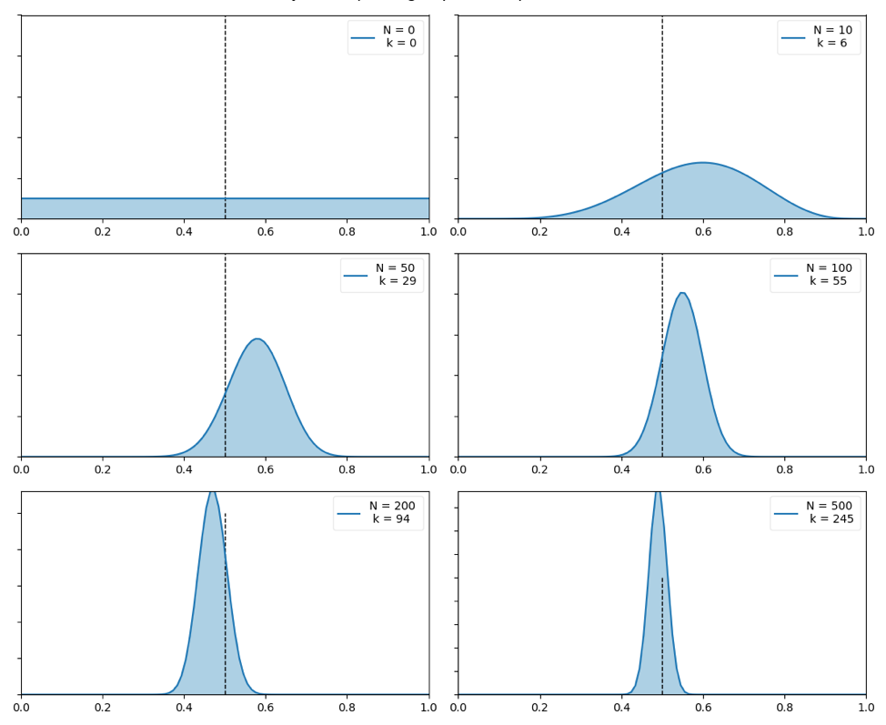
Figure 4 - Change of posterior distributions when increasing the test trials.

Figure 4 shows the change of posterior distribution as the availability of evidence increases. The data from Table 2 was used to plot the graphs in Figure 4.

• Each graph shows a probability distribution of the probability of observing heads after a certain number of tests. The x-axis is the probability of heads and the y-axis is the density of observing the probability values in the x-axis (see probability density functions).
• We start the experiment without any past information regarding the fairness of the given coin, and therefore the first prior is represented as an uninformative distribution in order to minimize the influence of the prior to the posterior distribution. Notice that even though I could have used our belief that the coins are fair unless they are made biased, I used an uninformative prior in order to generalize our example into the cases that lack strong beliefs instead.
• We flip the coin $10$ times and observe heads for $6$ times. We then update the prior/belief with observed evidence and get the new posterior distribution. Now the probability distribution is a curve with higher density at $\theta = 0.6$. Unlike in uninformative priors, the curve has limited width covering with only a range of $\theta$ values. This width of the curve is proportional to the uncertainty. Since only a limited amount of information is available (test results of $10$ coin flip trials), you can observe that the uncertainty of $\theta$ is very high.
• We updated the posterior distribution again and observed $29$ heads for $50$ coin flips. Now the posterior distribution is shifting towards to $\theta = 0.5$, which is considered as the value of $\theta$ for a fair coin. Moreover, notice that the curve is becoming narrower. This indicates that the confidence of the posterior distribution has increased compared to the previous graph (with $N=10$ and $k=6$) by adding more evidence.
• When we have more evidence, the previous posteriori distribution becomes the new prior distribution (belief). We can update these prior distributions incrementally with more evidence and finally achieve a posteriori distribution with higher confidence that is tightened around the posterior probability which is closer to $\theta = 0.5$ as shown in Figure 4.

As such, Bayesian learning is capable of incrementally updating the posterior distribution whenever new evidence is made available while improving the confidence of the estimated posteriors with each update.

Conclusion

The Bayesian way of thinking illustrates the way of incorporating the prior belief and incrementally updating the prior probabilities whenever more evidence is available. Moreover, we can use concepts such as confidence interval to measure the confidence of the posterior probability. Unlike frequentist statistics, we can end the experiment when we have obtained results with sufficient confidence for the task.

Even though frequentist methods are known to have some drawbacks, these concepts are nevertheless widely used in many machine learning applications (e.g. Lasso regression, expectation-maximization algorithms, and Maximum likelihood estimation, etc). Bayesian learning and the frequentist method can also be considered as two ways of looking at the tasks of estimating values of unknown parameters given some observations caused by those parameters. For certain tasks, either the concept of uncertainty is meaningless or interpreting prior beliefs is too complex. In such cases, frequentist methods are more convenient and we do not require Bayesian learning with all the extra effort. However, most real-world applications appreciate concepts such as uncertainty and incremental learning, and such applications can greatly benefit from Bayesian learning.

This blog provides you with a better understanding of Bayesian learning and how it differs from frequentist methods. In my next blog post, I explain how we can interpret machine learning models as probabilistic models and use Bayesian learning to infer the unknown parameters of these models.