
Bayesian Learning for Machine Learning: Part II - Linear Regression
Part I of this article series provides an introduction to Bayesian learning. With that understanding, we will continue the journey to represent machine learning models as probabilistic models. Once we have represented our classical machine learning model as probabilistic models with random variables, we can use Bayesian learning to infer the unknown model parameters. Such a process of learning unknown parameters of a model is known as Bayesian inference.
In this blog, first, we will briefly discuss the importance of Bayesian learning for machine learning. Then, we will move on to interpreting machine learning models as probabilistic models. I will use the simple linear regression model to elaborate on how such a representation is derived to perform Bayesian learning as a machine learning technique.
Why Bayesian learning?
In recent years, Bayesian learning has been widely adopted and even proven to be more powerful than other machine learning techniques. For example, we have seen that recent competition winners are using Bayesian learning to come up with state-of-the-art solutions to win certain machine learning challenges:
- March Machine Learning Mania (2017) - 1st place (Used Bayesian logistic regression model)
- Observing Dark Worlds (2012) - 1st and 2nd place
This shows that Bayesian learning is the solution for cases where probabilistic modeling is more convenient and traditional machine learning techniques fail to provide state-of-the-art solutions. Bayesian-based approaches play a significant role in data science owing to the following unique capabilities:
- Incorporating prior knowledge or beliefs with the observed data to determine the final posterior probability
- New observations or evidence can incrementally improve the estimated posterior probability
- The ability to express uncertainty in predictions
Let’s see why the above capabilities are important in machine learning, especially in real-world applications.
- One of the major challenges in machine learning is to prevent the model from overfitting. Especially when we have small datasets, the model will only learn the specific configurations of the given data that does not generalize to the unseen data. However, if we have beliefs that were gained through past experience, those could be used to generalize our models in the absence of a sufficiently large dataset. Therefore, with Bayesian learning, we can use such prior knowledge or beliefs to provide additional information to the models.
- Recently, the scalability of machine learning algorithms to big data applications has become a challenge due to limited computational resources. If a machine learning algorithm requires a complete dataset to be available in the memory for the computations, then those algorithms will require a large amount of memory to scale them to big data applications. However, if a machine learning algorithm can inherently support incremental learning, then, we can load a subset of the data into the memory for computations in each increment. Bayesian learning can be used as an incremental learning technique to update the prior belief whenever new evidence is available.
- The ability to express the uncertainty of predictions is one of the most important capabilities of Bayesian learning. Even though uncertainty is underappreciated in machine learning, it has significant benefits to real-world applications. The uncertainty of predictions is an important concept when making decisions involved with high risks in industries such as financial and medical industries.
Bayesian learning is now used in a wide range of machine learning models such as,
- Regression models (e.g. linear, logistic, poisson)
- Hierarchical Regression models (e.g. linear mixed effect, pooled/hierarchical regression)
- Mixture models (e.g. Gaussian Mixture models)
- Deep exponential families (e.g., deep latent Gaussian models)
- Linear dynamical systems (e.g., state space models, hidden Markov models)
- Gaussian process models (e.g., regression / classification)
- Topic models (e.g Latent Dirichlet allocation)
Even state-of-the-art techniques such as deep learning (Bayesian Deep Learning) and reinforcement learning (Bayesian Reinforcement Learning) use Bayesian learning to model probabilistic behavior, while facilitating the uncertainty of predictions (we discussed how to use Bayesian learning to model uncertainty in part I). This article explains why Bayesian learning is important for deep learning techniques, which are considered state of the art for a wide range of applications, such as image recognition/classification, automated driving, speech or text processing, and artificial intelligence (AI).
Our First Model
One of the simplest machine learning models is the simple linear regression model. Therefore, we can start with that and try to interpret that in terms of Bayesian learning. The simple linear regression tries to fit the relationship between dependent variable $Y$ and single predictor (independent) variable $X$ into a straight line. We can write that linear relationship as:
\begin{equation} \tag{1}
y_i = \tau + w.x_i+ \epsilon_i
\end{equation}
Here $\tau$ is the intercept and $w$ is the coefficient of the predictor variable. The term $\epsilon_i$ represents the individual error when modeling real-world data that does not fit perfectly to a straight line. Now we have to determine the values for these unknown parameters $\tau$ and $w$ minimizing the total error. One way of doing so is by minimizing the least squared error or using the maximum likelihood, which is categorized as frequentist methods. However, in Bayesian learning, we are not satisfied with a single point estimation, instead, we want to know the probability distributions of the unknown model parameters.
Regression Using the Frequentist Method
We discussed the frequentist method and how it differs from Bayesian learning in my first blog. Now let's try to see how we are using the frequentist method to find the unknown parameters of the simple linear regression model.
According to the frequentist method, we can determine a single value per each parameter ($\tau$ and $w$) for the linear regression model and find the best-fitted regression line by minimizing the error $\sum_{i=1}^{N} \epsilon_i$ for $N$ data points. We can use least squares and maximum likelihood to find such a regression line when using frequentist inference. I will not discuss in detail how such frequentist inference is performed. Instead, we will discuss the properties of the outcome of such classical machine learning techniques.
The following figure shows such a regression model for an artificially generated dataset. Note that here we have to determine a single coefficient $w$ and the intercept $\tau$; therefore, we can model the data and the dependent variable in the 2D space.
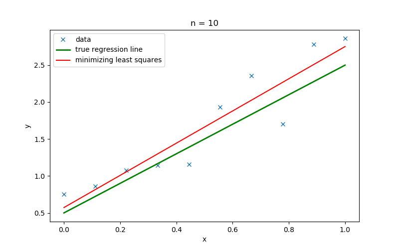
Figure 1: Linear regression lines for generated datasets with number of samples ($n$) $10$ and $100$
Figure 1 shows the linear regression lines that were inferred using minimizing least squares (a frequentist method) for a dataset with the number of samples ($n$) $10$ and $100$, respectively. When generating the dataset, the slope $w$ and the intercept $\tau$ was set to $2$ and $0.5$, respectively.
- We can see the regression line obtained minimizing least squares provides us a single regression line specific for the given data. However, this can lead to overfitting of the model. In Figure 1, when the number of samples is $10$, then the regression line drawn for those data is too specific to that dataset. Therefore, it significantly deviates from the true regression line. When more samples are available ($n=100$), we get a different regression line that is specific to the currently available information. Therefore, appropriate regularization techniques should be followed explicitly in order to increase the generalization of the model.
- Moreover, the frequentist method gives exact point estimations to the unknown model parameters ($w$ and $\tau$) and does not show the variation of those model parameters. In particular, if we do not have sufficient data, then we do not have a way of determining the uncertainty of the model parameters or the confidence attached to each parameter. We may assume that predictions using the regression line drawn using $100$ samples are more certain than the predictions from the regression line that is inferred with $10$ samples, yet we can’t measure the level of confidence attached to each prediction.
- Assume that before training the model, we knew that the slope $w$ of data is closer to $2$ due to some prior experience. Yet with the frequentist method, we can’t incorporate such knowledge when training the model.
Why Can't We Use Confidence Intervals to Estimate Uncertainty?
Even though we can compute the confidence intervals using frequestis statistics for the estimated values, notice that confidence interval is not equivalent to the uncertainty. Confidence interval guarantees with a certain confidence that the estimated value lies within a certain interval, whereas concepts of uncertainty in Bayesian learning measures the confidence of the each value from the estimated posterior distributions.
Implementing the First Bayesian Model
In Bayesian learning, we represent variables as random variables with probability distributions. Let’s try to convert the classical linear regression model that we discussed above into a Bayesian linear regression model.
However, for the impatient, first, I’ll present the implementation of such a Bayesian linear regression model using the Python language and the PyMC3 probabilistic programming framework.
# training the model
# model specifications in PyMC3 are wrapped in a with-statement
with pm.Model() as model:
   # Define priors
   x_coeff = pm.Normal('x', 0, sd=20)  # prior for coefficient of x
   intercept = pm.Normal('Intercept', 0, sd=20)  # prior for the intercept
   sigma = pm.HalfCauchy('sigma', beta=10)  # prior for the error term of due to the noise

   mu = intercept + x_coeff * shared_x  # represent the linear regression relationship

   # Define likelihood
   likelihood = pm.Normal('y', mu=mu, sd=sigma, observed=y_train)

   # Inference!
   trace = pm.sample(1000, njobs=1)  # draw 3000 posterior samples using NUTS sampling
In PyMC3, we have to include the specification of model architecture within a with statement. Inside the with statement, we define the random variables of our model. Here we have defined three prior distributions corresponding to each unknown variable in the linear regression model:
- Coefficient of $x$ (x_coeff) - Normal distribution
- Intercept - Normal distribution
- Error term (sigma) - Half Cauchy distribution
The choice of distribution and their parameters of the priors are simply based on our beliefs and past experience. Assume if we have seen that for similar cases, the probability distribution of the intercept follows a normal distribution with parameters $\mu=2$ and $\sigma^2 = 1$. Then, we can reduce the effort taken to determine the posterior of intercept during training by incorporating that information when defining the prior of the intercept. The ability to incorporate our beliefs into the model is a major advantage of using Bayesian learning for implementing machine learning models. However, a bad choice of prior can lead to poor models or to situations even worse than classical models without priors. In the above implementation, we have selected priors simply by considering the nature of each parameter (i.e., the error term/sigma is given a Half Cauchy distribution since it is considered the variance of the likelihood). Since this is a simple model with three unknowns, we expect any inconsistencies in our priors to be eliminated during the training.
Once we have defined the priors, we need to specify the likelihood of our model. The shape and the parameters of the distributions of the likelihood can be used determine the type of the model. In the above script, the likelihood is defined as a normal distribution with mean $w.x_i+\tau$. Therefore, the mean of the likelihood connects the independent variable $x_i$ and the dependent variable $y_i$ forming a linear regression model. Furthermore, a random variable that represents the error term is used to define the standard deviation of that normal likelihood. Then, we include our observations to the likelihood using the observed argument of the PyMC3 distributions.
Let's try to further understand how likelihood can be used to determine the type of model. Assume instead a linear regression model; we are required to implement a logistic regression model for binary classification using the below relationship between the dependent variable $y_i$ and the independent variable $x_i$.
$$y_i =sigmoid(w.x_i + \tau)$$
It should be noted that this logistic regression model also require estimating the coefficient and the intercept; therefore, let’s assume the priors of those unknowns follow the same distributions as the corresponding prior to the linear regression model. However, we can’t use the normal likelihood anymore, since the likelihood of logistic regression is a discrete random variable. Instead, we use the Bernoulli likelihood, which is used to represent the observation from a single trial experiment that has only two possible outcomes (yes/no and 1/0 etc). Therefore, we can modify the above linear regression model to a logistic regression model by simply replacing the normal likelihood with the Bernoulli likelihood with a $p$ value $sigmoid(w.x_i + \tau)$ as shown below.
p = sigmoid(intercept + x * w)
# Define likelihood
likelihood = pm.Bernoulli('y', p=p, observed=y_train)
Finally, we use the PyMC3 sample method to perform Bayesian inference through sampling the posterior distributions of three unknown parameters. By default, PyMC3 uses NUTS to decide the sampling steps. Let’s discuss different Bayesian inferences techniques and some of the MCMC samplers in another blog, the focus in this article will be to understand the underlying concepts that are used to define Bayesian models.
The full code for the both Bayesian linear and logistic regression using Python and PyMC3 can be found using this link, including the script for the plots.
Understanding the Model
Even though we discussed the implementation of the Bayesian regression model, I skipped the fun parts where we try to understand the underlying concepts of the above model. You should now have many questions, such as how did I decide the values for the parameters of the likelihood and how does the above model architecture adhere to the Bayes’ rule we learnt in the first article, etc? Let’s try to resolve these questions while trying to understand the above model with probabilistic concepts.
In Bayesian learning, we consider each observation $y_i$ as a probability distribution, in order to model the both observed value and the noise of the observation. Let’s assume that each observation $y_i$ is distributed normally as shown below.
\begin{equation} \tag{2}
y_i \sim \mathcal{N}(\mu_i, \sigma^2)
\end{equation}
Here, we have defined that each observation $y_i$ follows a normal distribution with a mean $\mu_i$ and a variance $\sigma^2$. Now, let’s try to understand the meaning of these $\mu_i$ and $\sigma^2$ in terms of the linear regression model. We know that mean of a normal distribution is the most probable value for that random variable. However, according to the linear regression equation, we believe that $w.x_i + \tau$ is the most probable value for $y_i$. Therefore, we can define $\mu_i$ as,
\begin{equation} \tag{3}
\mu_i = w.x_i + \tau
\end{equation}
Even though $\mu_i$ is the most probable value for $y_i$, $y_i$ can also include some error or noise. Accordingly, we model such errors $\epsilon_i$ in the observations by adjusting the variance term $\sigma^2$ to compensate for the deviations of $y_i$ from $\mu_i$. Let’s denote the error term $\epsilon$ using a normal distribution with a zero mean and $\sigma^2$ variance.
\begin{equation} \tag{4}
\epsilon \sim \mathcal{N}(0, \sigma^2)
\end{equation}
If we add a constant $\mu_i$ to the normal distribution shown by equation 4, we get a new normal distribution with a mean $\mu_i$ and variance $\sigma^2$, which is the likelihood of the observation $y_i$.
\begin{equation} \tag{5}
y_i \sim \mathcal{N}( w.x_i + \tau , \sigma^2)
\end{equation}
Now you should be able to understand how each term in the traditional linear regression model (equation 1) is represented using the normal distribution as shown in equation 5. Even if we think for a moment, the mean and the variance of a normal distribution represent the most significant value and the deviation of the values from that most significant value, respectively. Moreover, the values nearby the mean will have a higher chance of appearing, whereas the probability of observing the value reduces when moving away from the mean. Therefore, our assumption to choose a normal distribution to represent the random variable $y_i$ is not an arbitrary decision, it is chosen such that we can represent the relationship between the dependent variable $y_i$ and independent variables $x_i$ with the effect of the error term $\epsilon_i$ using the properties of the normal distribution.
Once we define the linear regression model using the notation shown in equation 5, we get three unknowns: $w$, $\tau$ and $\sigma^2$ . It should be noted that even though the $mu_i$ is considered as a deterministic variable, it is derived using the unknowns $w$, $\tau$ (equation 3). In Bayesian learning, these unknowns are also called as hidden or latent variables, because we have not seen values of those variables yet. Therefore, we have to determine the parameters $w$, $\tau$ and $\sigma^2$ using Bayesian inference given the $X$ and $Y$. We can represent such relationships between random variables using the conditional probability distribution $P(w, \tau, \sigma^2 | Y, X) $.
If we apply the Bayes’ theorem to $P(w, \tau, \sigma^2 | Y, X) $, we get the following expression,
\begin{equation} \tag{6}
\underbrace{P(w, \tau, \sigma^2 | Y, X)}_{\text{posterior}} = \frac { \underbrace{P(Y|w, \tau, \sigma^2, X)}_{\text{likelihood}}\underbrace{P(w, \tau, \sigma^2)}_{\text{prior}} } {\underbrace{P(Y|X)}_{\text{evidence}}}
\end{equation}
We are trying to determine the parameters of the linear regression model, and therefore we can rewrite the above general expression specific to the linear regression model. Notice that we have omitted the evidence $P(Y|X)$ in following equations in order to simply the equations.
\begin{equation} \tag{7}
P(w, \tau, \sigma^2 | Y, X) \propto P(Y|w.X + \tau, \sigma^2)P(w, \tau, \sigma^2)
\end{equation}
Assuming that $w$, $\tau$ and $\sigma^2$ are conditionally independent and observations $y_i$ are conditionally independent of each other, we can rewrite the above equation for N data points as follows,
\begin{equation} \tag{8}
P(w, \tau, \sigma^2 | Y, X) \propto \prod_{i=1}^N [P(y_i|w.x_i + \tau, \sigma^2)]P(w)P(\tau)P(\sigma^2)
\end{equation}
If we can determine the posterior distributions of the hidden variables, then we can determine the values for those parameters with a certain confidence. First, we have to define the prior probability distributions for those unknown parameters.
\begin{align}
P(w) &= \mathcal{N}(w| \mu_1, \sigma^2_1) \nonumber\\
P(\tau) &= \mathcal{N}(\tau| \mu_2, \sigma^2_2) \nonumber\\
P(\sigma^2) &= \mathcal{HC}(\sigma^2|\beta)
\tag{9} \end{align}
As shown in equation 9, we have chosen the shape of the probability distributions for $w$ and $\tau$ to be normally distributed and we have given $\sigma^2$ the Half-Cauchy distribution. One could say this is our prior belief regarding those parameters. Actually, we have no way of deciding the perfect distribution to represent our prior belief for this case, yet we assume that those random variables can be modeled using the normal distribution. The $\mu_1$, $\sigma^2_1$, $\mu_2$, $\sigma^2_2$ and $\beta$ are the hyperparameters to the model, which are also considered as a part of prior belief. Even though it is difficult to determine the shape of the unknown model parameters, we can still guess reasonable values for some of the above hyperparameters. For example, in the above single coefficient dataset (Figure 1), if the $y_i$ values are $10$ times larger than the $x_i$ values, then selecting $\mu_1 = 1$ does not make any sense. Since $y_i \approx 10 \times x_i$, the most probable value for $w$ should be closer to $10$ and, therefore, we could choose the mean $\mu_1 = 10$ . However, we expect the influence of these hyperparameters to the model to be insignificant when provided with sufficient evidence to update the prior distributions (recall the coin-flip example).
Since we have defined the prior probability distributions, now it is time to define the likelihood of the model. The likelihood of the linear regression model is the probability of $y_i$ given $w.x_i + \tau$ and \sigma^2. We have already defined $y_i$ in terms of $w$, $\tau$ and $\sigma^2$ in the equation 5. Therefore the likelihood is given by:
\begin{equation} \tag{10} P(y_i|w.x_i+\tau,\sigma^2) = \mathcal{N}(y_i|w.x_i+\tau, \sigma^2)\end{equation}
Now, we have defined all the components of the linear regression model using random variables with probability distributions. Let’s rewrite the posterior distribution using the likelihood and prior distributions that we have defined above.
\begin{align}
P(w, \tau,\sigma^2| Y, X) =
\frac{\prod_{i=1}^N [\mathcal{N}(y_i|w.x_i+\tau, \sigma^2)]\mathcal{N}(w|\mu_1, \sigma^2_1) \mathcal{N}(\tau|\mu_2, \sigma^2_2)\mathcal{HC}(\sigma^2|\beta)}{P(Y|X)}
\tag{11} \end{align}
Equation 11 defines the Bayesian model for the simple linear regression model. Now we can call this the Bayesian linear regression model. By using the model shown above, we can determine the joint posterior probability distribution of $w$, $\tau$ and $\sigma^2$. As I have mentioned earlier, the process of learning hidden variables is called Bayesian inference. I will discuss some of those techniques that are used for Bayesian inference in my next article. However, let’s try to understand the properties of the models trained using Bayesian inference by looking at a simple linear regression model trained using the artificially generated dataset shown in Figure 1.
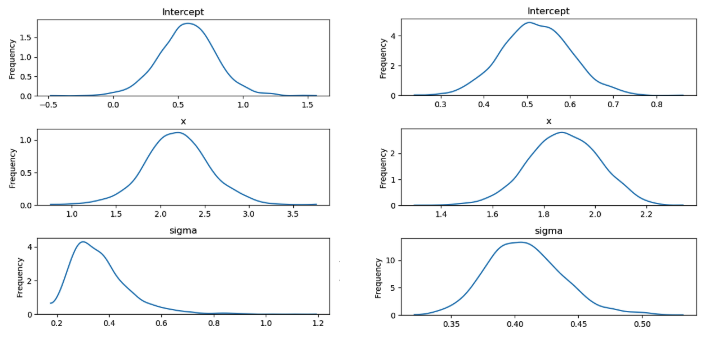
Figure 2: The posterior probability distributions of $tau$, $w$ and $sigma^2$ (for$ n = 10$ and $n = 100$, respectively)
In Figure 2, we can observe that instead of exact point estimations, now we have probability distributions for each model parameter. Even though we started with normal priors for hidden parameters ($w$ and $\tau$), the posterior distributions have a different shape. However, we used a Half-Cauchy prior for the $\sigma^2$, yet the posterior distribution of that is closer to the normal distribution. Therefore, even with the poor choice of priors, we can achieve accurate posteriors if sufficient evidence/data is available (notice the change of $\sigma^2$ from $n=10$ to $n=100$). However, it should be noted that poor priors should be avoided since they could affect the accuracy of the models significantly in the absence of sufficient data. Furthermore, if we have fairly accurate priors, we can achieve better results even with fewer data, whereas frequentist methods lead to overfitting of models with fewer data. Moreover, with more and more data, the slope ($w$) and the intercept ($\tau$) are getting closer to the real values. The confidence of the estimated parameters is increased (compare the width of curves between $n=10$ to $n=100$) when more information is provided to learn the parameters.
The following diagram shows multiple regression lines that were plotted using the samples extracted from such posterior distribution for the artificially generated data set.


Figure 3: Posterior predictive regression lines (for $n=10$ and $n=100$)
Here, each black line corresponds to a single pair from both $w$ and $\tau$ that was sampled from their estimated posterior distributions. The green line is the true regression line. When we have less data (for $n=10$), the regression lines inferred using Bayesian learning are widely spread due to the high uncertainty of the model, whereas the regression lines are well packed together closely to the true regression line when we have provided more information ($n=100$) to train the model.
Predictions from Bayesian Models
The models are useless if we don’t know how to make predictions using them (unless we have trained the models for a different purpose). Therefore, I wanted to make some comments on how to make predictions using Bayesian models.
Given a new independent value $\bar{x}_i $, we want to predict the value of unseen $\bar{y}_i $ using the model that we have trained with previous data $D={X,Y}$. Using the trained model, we determine the predictive distribution which is the probability distribution of $\bar{y}_i $. Since we can obtain a probability distribution for each prediction, we get uncertainty of the predictions for free. We can derive the predictive distribution of above linear regression model as follows,
\begin{align}
P(\bar{y}_i | \bar{x}_i, D) = &\int_w \int_\tau P(\bar{y}_i, w, \tau | \bar{x}_i, D) \mathrm{d} w \mathrm{d}\tau &&\text{law of total probability} \nonumber \\
=& \int_w \int_\tau P(\bar{y}_i | \bar{x}_i, w, \tau).P(w, \tau |D) \mathrm{d} w \mathrm{d}\tau &&\text{the product rule} \nonumber \\
=& \int_w \int_\tau P(\bar{y}_i | \bar{x}_i, w, \tau).P(w|D).P(\tau|D) \mathrm{d} w \mathrm{d}\tau &&\text{assuming conditionally independency}
\tag{12} \end{align}
Even though the equation for general predictive distribution is written in terms of $\bar{x}_i$ and data $D$, we have derived an expression for predictive distribution by replacing the term for data ($D$). It should be noted that $P(w|D)$ and $P(\tau|D)$ are the posterior distribution $P(w|Y,X)$ and $(\tau|Y,X)$ that were estimated during the training.


Figure 4: Predictions using regression models (for$ n=10$ and $n=100$)
In figure 4, we can see the predictions using Bayesian and frequentist linear regression models. However, the Bayesian regression model is capable of determining the uncertainty of each prediction rather than just producing the predictions. If we consider the plot corresponding to n=10, the uncertainty of predictions increases with the distance between the prediction and the true regression line (predictions closer to the true regression line has slightly small error bars compared to the predictions far away from the true regressor). Moreover, when increasing the number of data points, the model is further improved to produce more accurate predictions with higher confidence (notice the small error bars when $n=100$ compared to $n=10$).
Typically, classical machine learning models are less useful in the absence of sufficient data to train those models. However, a Bayesian model can still be useful with less data owing to its capability to attach an uncertainty value with each prediction. Moreover, if we have beliefs or past experience regarding the unknown parameters, then, we can use them as priors to the model in order to compensate for the missing data. Furthermore, we can incrementally update the models when more data is available rather than creating a new model to include each piece of information.
A Small Note on Bayesian Inference
Now we know how to represent machine learning models as probabilistic models and interpret them using the Bayes’ theorem. However, we still did not discuss how to perform Bayesian inference in order to determine the posterior distributions of the unknown parameters given the priors and the observations (data).
In upcoming articles, I will introduce such Bayesian inferences techniques and then provide an in-detail discussion of commonly used Bayesian inferences techniques such as Markov Chain Monte Carlo (MCMC) sampling and Variational Inferences. However, I’ll present a challenge for you, before reading the next article, you can try to come up with your own algorithm to perform the Bayesian inference for the simple linear regression model discussed above.
Conclusion
We discussed how to interpret the simple linear regression in the context of Bayesian learning in order to determine the probability distributions of the unknown parameters rather than exact point estimations for those parameters. The Bayesian regression model that we discussed above can be extended for other types of models (such as logistic regression and Gaussian mixtures etc) by defining the priors for random variables and the likelihood as probability distributions and then mapping those random variables to exhibit the properties of the desired model. In fact, you can model any type of relationship between independent variables and dependent variables, then let Bayesian inferences figure out the inference of those parameters. Moreover, the uncertainty attached with each prediction enhance the decision making to make more safe and accurate decisions, while the incremental updates to the priors can improve the confidence and the accuracy of the predictions when more information is available.